
Extraction of bipolar SPICE Gummel-Poon parameters related to reverse Gummel (Ie and Ib vs. Vbc) 
Theory
Introduction:
BJT Parameter Extraction from Reverse Gummel Plots
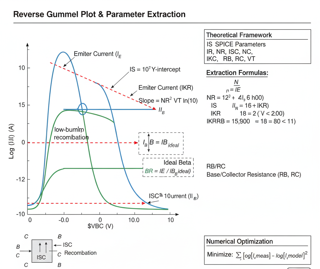
Fig. 1. Reverse Gummel Plot & Parameter Extraction
Introduction
The reverse Gummel plot is the counterpart to the forward Gummel plot. It is essential for extracting the parameters that govern the BJT's operation in the reverse-active and saturation regions.
A reverse Gummel plot is generated by plotting the emitter current ($I_E$) and base current ($I_B$) on a logarithmic scale against the base-collector voltage ($V_{BC}$) on a linear scale. During this measurement, the base-emitter voltage is held constant at zero ($V_{BE} = 0$).
This measurement configuration effectively operates the transistor "backwards," with the collector acting as the emitter and the emitter acting as the collector.
The Gummel-Poon Model (Reverse Active)
With $V_{BE} = 0$, the forward-active terms in the Gummel-Poon model become negligible. The model simplifies to describe the reverse-active operation:
$$ I_E \approx \frac{IS}{q_b} \cdot \left( e^{\frac{V_{BC}}{NR \cdot V_T}} - 1 \right) $$
$$ I_B \approx \left[ \frac{IS}{BR} \cdot \left( e^{\frac{V_{BC}}{NR \cdot V_T}} - 1 \right) \right] + \left[ ISC \cdot \left( e^{\frac{V_{BC}}{NC \cdot V_T}} - 1 \right) \right] $$
Where the key reverse-mode parameters are:
- $IS$: Transport Saturation Current (the same as in the forward model, per reciprocity).
- $BR$: Ideal Maximum Reverse Beta.
- $NR$: Reverse Current Emission Coefficient (ideality factor for $I_E$).
- $ISC$: Base-Collector Leakage Saturation Current.
- $NC$: Base-Collector Leakage Emission Coefficient (ideality factor for non-ideal $I_B$).
- $q_b$: Normalized base charge, which includes high-injection effects modeled by
IKR. - $V_T$: Thermal Voltage ($kT/q$).
Graphical Extraction from Plot Regions
Similar to the forward plot, we analyze the different regions of the reverse Gummel plot.
1. Ideal Mid-Current Region
In this region, $I_E$ and the ideal component of $I_B$ are dominated by diffusion. They appear as parallel straight lines.
IS(Transport Saturation Current): Extrapolate the linear (ideal) portion of the $log(I_E)$ curve back to its intercept at $V_{BC} = 0$. Due to the Ebers-Moll reciprocity principle, this value must be the sameISextracted from the forward Gummel plot's $I_C$ curve. This provides a critical consistency check. $IS = 10^{\text{intercept}}$NR(Reverse Emission Coefficient): Find the slope of the linear (ideal) portion of the $log(I_E)$ curve. $\text{Slope}{IE} = \frac{\Delta \log{10}(I_E)}{\Delta V_{BC}} = \frac{1}{NR \cdot V_T \cdot \ln(10)}$NRis typically very close to 1.0.BR(Ideal Maximum Reverse Beta): This is the ideal current gain in the reverse-active mode. It is found from the vertical separation between the ideal $I_E$ line and the (extrapolated) ideal $I_B$ line. $BR = \frac{I_E}{I_{B, \text{ideal}}}$ For standard asymmetric BJTs (where the emitter is much more heavily doped than the collector),BRis very small (e.g., 0.1 to 5). This means the $log(I_E)$ and $log(I_B)$ curves will be very close together in this region.
2. Low-Current Region
At low $V_{BC}$, the non-ideal recombination current in the base-collector space-charge region dominates the base current $I_B$.
NC(B-C Leakage Emission Coefficient): The $log(I_B)$ curve deviates from the ideal $N=1$ slope and follows a new, shallower slope. Find the slope of this line. $\text{Slope}{IB} = \frac{\Delta \log{10}(I_B)}{\Delta V_{BC}} = \frac{1}{NC \cdot V_T \cdot \ln(10)}$NCis typically between 1.5 and 2.0.ISC(B-C Leakage Saturation Current): Extrapolate this non-ideal (low-current) $log(I_B)$ line back to its intercept at $V_{BC} = 0$. $ISC = 10^{\text{intercept}}$ Since the B-C junction area is typically much larger than the B-E junction area,ISCis usually much larger thanISE.
3. High-Current Region (Roll-off)
At high $V_{BC}$ and high currents, the curves "roll off" due to high-level injection and parasitic resistances.
IKR(Reverse High-Injection Knee): This is the "knee" in the $log(I_E)$ curve where its slope decreases. It models high-level injection in the collector region (which is acting as the emitter).IKRis the approximate emitter current at this knee.IKRis typically much smaller than its forward counterpartIKF.Parasitic Resistances (
RB,RC): These resistances cause voltage drops that reduce the internal junction voltages.RB(Base Resistance): The $I_B \cdot RB$ drop causes the $log(I_B)$ curve to roll off.RC(Collector Resistance): The $I_E \cdot RC$ drop (since $I_E \approx I_C$ in this mode) is often the dominant resistive effect, causing both $I_E$ and $I_B$ curves to roll off.
Summary
The reverse Gummel plot is critical for modeling saturation. The parameters extracted (BR, ISC, NC, IKR) are essential for any simulation where the BJT's base-collector junction becomes forward-biased, which is common in digital logic (ECL, TTL) and analog switching applications.