Step 1: Understanding the Interface

Open the simulation and familiarize yourself with the control panels:

• Left Panel: Wavepacket Parameters and Potential Barrier controls
• Center: Visualization canvas showing the quantum wavefunction
• Right Panel: Learning Scenarios and Physics Data

---

Step 2: Set Initial Parameters

Parameter	Recommended Initial Value	Purpose
Particle Energy (E)	0.030	Energy of incoming wavepacket
Barrier Height (V₀)	0.040	Height of potential barrier
Barrier Width (L)	20	Width of the barrier region
Ramp Gradient	0	Keep sharp edges initially

---

Step 3: Start the Simulation

1. Click the ▶️ Play button to start the animation
2. Observe the wavepacket moving towards the barrier
3. Watch the Reflected % and Transmitted % values change in real-time.

---

Step 4: Explore Learning Scenarios

Try each preset scenario from the right panel:

1. 🟢 Easy Tunnel - Observe high transmission
2. 🟡 Balanced - See wave splitting
3. 🔴 Hard Tunnel - Notice low transmission
4. 📚 Classical - Compare with classical behavior
5. 📏 Wide Barrier - Observe exponential decay
6. 📶 Step Potential - Study step function behavior

---

Step 5: Display Options

Use the display options in the visualization panel:

• Density: Shows probability density |Ψ|² with phase as color
• View: Shows Real and Imaginary parts of the wavefunction
• Grid: Enable grid for reference measurements

---

Step 6: Collect Data

Record your observations in the table below:

S.No	Particle Energy (E)	Barrier Height (V₀)	Barrier Width (L)	Transmission %	Reflection %
1	0.030	0.040	20	1.04%	98.96%
2	0.060	0.020	15	96.79%	3.21%
3	0.035	0.035	25	8.38%	91.62%
4	0.020	0.050	30	≈ 0.00%	≈ 100.00%
5	0.070	0.050	10	73.04%	26.96%
6	0.045	0.030	40	89.25%	10.75%

---

Step 7: Analyze the Effect of Barrier Width

Keep E and V₀ constant, vary only the Barrier Width (L):

S.No	Barrier Width (L)	Transmission %	Observation
1	10	16.69%	High transmission with thin barrier
2	20	1.04%	~16x drop from L=10 — exponential decay begins
3	30	0.062%	Exponential decay clearly observed (T ∝ e-2κL)
4	40	0.0037%	Very low transmission with thick barrier
5	50	0.0002%	Near-zero transmission, confirms T ∝ e-2κL

---

Step 8: Plot the Graph

Using your collected data, plot a graph with:

• X-axis: Barrier Width (L)
• Y-axis: Transmission Percentage (%)

Observe the exponential relationship: T ∝ e^-2κL

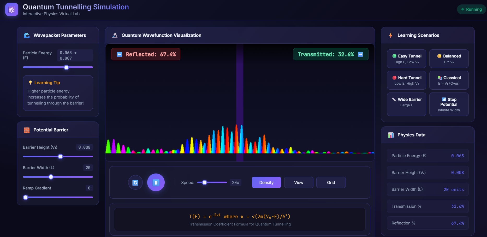
Fig.1 Quantum Wavefunction Visualization in Density form

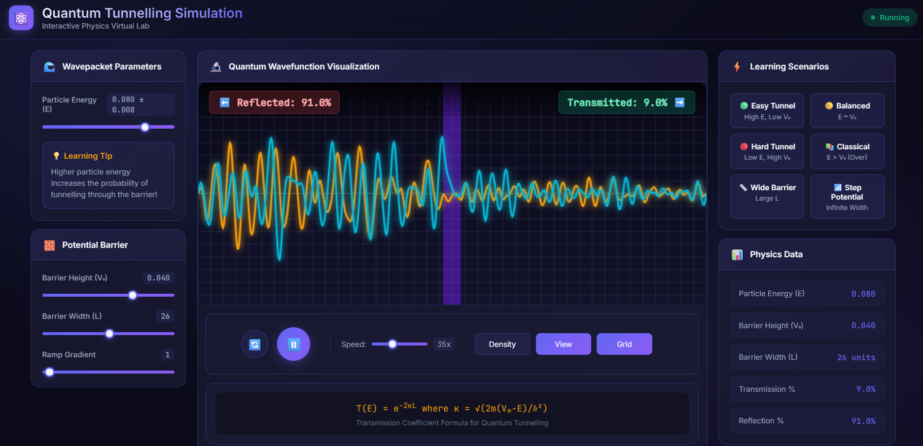
Fig.2 Quantum Wavefunction Visualization in frequency form

---

Step 9: Conclusions

Based on your observations, answer:

1. How does particle energy affect tunnelling probability?
2. How does barrier width affect transmission coefficient?
3. What happens when E > V₀ (classical regime)?
4. Why does tunnelling probability never become exactly zero?