As a metal/alloy solidifies from a melt, nuclei grow as a crystal until they impinge on a nearby growing crystal. The interface between this interfacing region is called as ‘grain boundary’ whereas the crystalline (or similarly aligned region) is called as a grain. Grain size plays a very important role in dictating the mechanical properties of a material, hence is makes sense to be able to quantify it. Quantification of grain size may permit linking the process parameters that result the same. Consequently, these parameters (such as cooling rate or superheat temperature or mold temperature, etc.) will provide fair indication of the grain size expected from such settings.

As one will observe the microstructure will comprise of grains (Figure 1a). Though the schematic provides very regular and similar grains, but in practical cases the grains are typically heterogenous in nature (Fig. 1b). Nonetheless, it is imperative that the grain size needs to be measured. So for a given magnification, a standard reticule (i.e. a scale/ruler with markings) is observed for setting up scale bar and then impressed on the image after due calibration (with image processing). Accordingly, Figure 2 presents such a microstructure, which is calibrated using the reticule and allows estimation of size of grain.

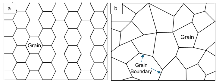
Figure 1: Schematic showing microstructure with: a) Homogeneous grains and size, and (b) Heterogenous grain size.

From the scale bar provided in Figure 2, now one can estimate the grain size to be ~13 µm. In other words, the insertion of scale bar has now provided the ability to ‘quantify’ the grain size. In this case, the grains are homogeneous and possess same grain size. But, in many cases the grains are heterogeneous and an average grain size, or grain distribution needs to be estimated.

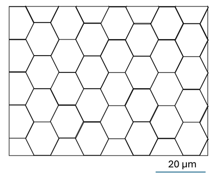
Figure 2: Schematic of microstructure with an inserted scale bar to estimate the grain size.

Grain Size Measurement:
There are multiple ways of estimating grain size. The first outlook is to ‘guess’ an estimate from the scale bar as the first observation. By a crude observation, the grain size in Figure 3 appears to be ~20 µm. But, with a different observer, the grain size may vary from 15-30 µm. So, estimations require standard methods of measuring grain size, sch as: (i) ASTM grain size, (ii) Jeffries method, (iii) Triple Point method, and (iv) Image Analysis (taken later as Experiment 10).

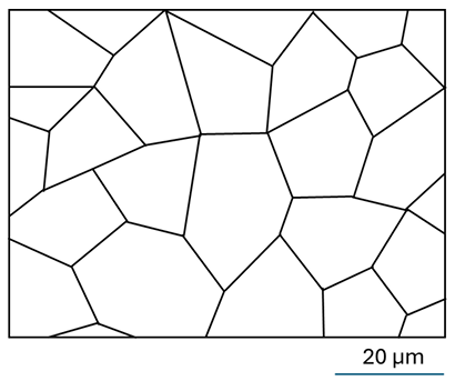
Figure 3: Grain size estimation in a microstructure with non-uniform grains.

(i) ASTM grain size measurement
ASTM grain size is given as :
N=2^n-1

where N is the number of grains at 100x in 1 in² area, and n is the ASTM Grain Size. If the grains are calculated in in2 area at 50× magnification, then as the area is reduced by 2 times along each of x and y-axes, the value of N should be divided by 2² (or 4) to obtain the number of grains that would be visible in that area at 100×. Similarly, if the magnification is say 500×, then each side is reduced by 5 times, and the number of grains at 100× would have been 5² (or 25 times) more at 100×. So, magnification should be properly accounted for (in 1 in² area) for estimating ASTM grain size.

It may also be noted that ‘Comparison method’ can also be used to visually compare the microstructure of a specimen to a series of graded images or charts of known grain sizes. Herein, a number of grain sizes are already provided, and whichever possesses very similar (known) grain size to the one experimentally prepared, can be compared to obtain grain size.

(ii) Jeffries Method:

In Jeffries method, a circle with an area of 5000 mm² is captured and number of grains are counted therein. The total of: (i) full grains (n₁), and (ii) half-count of grains intersected at circumference (n₂) are multiplied by Jeffries factor (f=M²/5000), where M is the magnification to obtain number of grains per mm² (N_A).

N_A = 𝑀²/5000 (𝑛₁+𝑛₂/2)

Now average grain area (Ā), with units of mm², is obtained as 1/N_A. For average grain area in µm²,

Ā (µm²) = 10⁶/N_A

Or mean diameter (d) is given as:
d̄(𝜇𝑚) = (𝐴̅)^1/2 = 10³/𝑁_A^1/2

As the ASTM grain size is given as :
N=2^n-1

Where N is the number of grains at 100x in 1 in² area, and n is the ASTM Grain Size. Or taking log both sides, we get

or log N = (n-1) log 2
or 𝑛 = (log𝑁/log2) + 1

If the grains are calculated in in2 area at 100 × magnification (for N), and need to be converted to per mm² at 1× magnification (N_A), then
N = N_A (25.4/100)²

Now n = (log N_A (25.4/100)² / log 2 ) + 1

n = (log N_A/ log 2 ) + log (25.4/100)² + 1

n = 3.32 log N_A − 3.95 + 1

n = 3.32 log N_A − 2.95

Please note that N_A is the number of grains in 1 mm² area at 1× magnification. Thus, now the ASTM grain size (n) can be calculated from number of grains per mm² at 1× magnification via Jeffries method.

(iii) Triple Point Method:

Grain boundary triple points (P) in an area are counted, and quadruple points (where four grains meet) is taken as ‘two units’.
Number of grains per unit area (N_A) is calculated using the equation:

N_A = (p/2) + 1 / A_T

where A_T is the area at 1× magnification.

The ASTM grain size, (n) is obtained as:
n = 3.322 log ((p/2) + 1 / A_T) - 2.95

Grain Boundary Measurement:
Grain boundary area per unit volume (G_A/V) is given as:

G_A/V = N/L

Where N is the number of intersections with grain boundary per unit length (L).

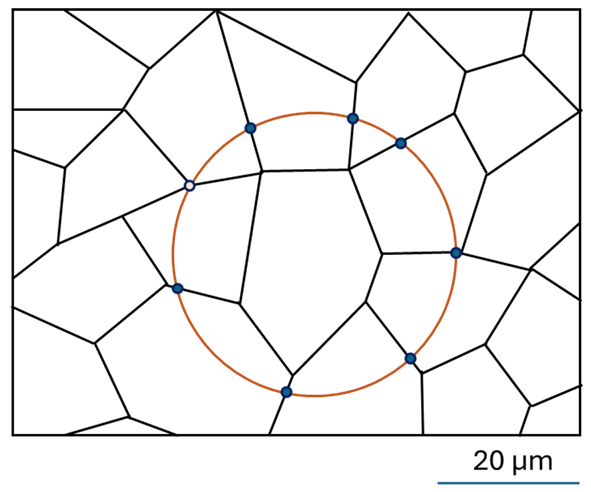
Figure 4: Grain boundary area intersections are marked with filled circles (weight of 1 each), whereas the triple point region is marked with a hollow circle (weight of 1.5)

From Figure 4, grain boundary area = {2×(1.5)+ 7)}/125.6 = 10/125.6
= 0.08/µm or 80 /mm or 80 mm²/mm³