Theory

The absolute stability and relative stability of the linear time-invariant continuous time closed-loop control system are determined by the location of the closed-loop poles in the S-plane. For example, complex closed-loop poles in the left half of the S-plane near the jω axis will exhibits oscillatory behavior, and closed-loop poles on the negative real axis will exhibit exponential decay.
Since the complex variables z and s are related by z = e^sT , the pole and zero locations in the Z-plane are related to the pole and zero locations in the S-plane. Therefore, the stability of the linear time-invariant discrete-time closed-loop system can be determined in terms of the locations of the poles of the closed-loop pulse transfer function. It is noted that the dynamic behavior of the discrete-time control system depends on the sampling period T. In other words, a change in the sampling period T modifies the pole and zero locations in the Z-plane and causes the response behavior to change.

Mapping of the Left Half of the S-plane into the Z-plane
In the design of a continuous-time control system, the locations of the poles and zeros in the S-plane are very important in predicting the dynamic behavior of the system. Similarly, in designing discrete-time control systems, the locations of the poles and zeros in the Z-plane are very important. Figure 1 shows the stable region in the s plane and its transformation into the z plane.

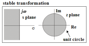
Fig.1. Mapping the stable region of s plane into z plane

When impulse sampling is incorporated into the process, the complex variables z and s are related by the equation:

$$ z = e^{sT} \tag{1} $$

This means that a pole in the s plane can be located in the z plane through the transformation. Since the complex variable s had real part σ and imaginary part ω, we have

$$ s = σ + j ω \tag{2} $$

and

$$ z = e^{T(σ +j ω)} = e^{T σ} e^{jT ω} = e^{T σ} e^{j(T ω + 2 πk)} \tag{3} $$

From this last equation we see that poles and zeros in the s plane, where frequencies differ in integral multiples of the sampling frequency 2 π/T , are mapped into the same location in the z plane. This means that there are infinitely many values of s for each value of z.

Since σ is negative in the left half of the s plane, the left half of the s plane corresponds to

$$ |z| = e^{T σ} \lt 1 \tag{4} $$

The j ω axis in the s plane corresponding to |z| = 1. That is, the imaginary axis in the s plane (the line σ = 0) corresponding to the unit circle in the z plane, and the interior of the unit circle corresponds to the left half of the s plane.

The exponential mapping forms the theoretical basis for several standard methods such as impulse invariance and bilinear transformation used in the conversion of analog systems to digital. The impulse invariance method directly uses this mapping to transform each pole of the analog system to the digital domain using the relation z = e^sT. This method preserves the time-domain impulse response of the system but may suffer from aliasing, especially when high-frequency components are present.
On the other hand, the bilinear transformation uses a rational approximation of the exponential mapping, given by:

$$ z = \frac{1+\frac{sT}{2}}{1-\frac{sT}{2}} $$