
Study and Operation of Inverted Pendulum System 
Theory
The inverted cart–pendulum is an example of under-actuated, non-minimum phase and highly unstable system.
The first step in the analysis of control system is to derive its mathematical model to understand the working of the complete system.
The Plant (Cart-Pendulum)
Pendulum set description
The pendulum setup consists of a cart moving along the 1 meter length track. Two pendulums are mounted on the cart’s shaft and are fixed together using an arm fixing screw.
As a result, they share the same angle of rotation (θ). The cart can move back and forth causing the pendulums to swing. The movement of the cart is caused by pulling the belt
in two directions by the dc motor attached at the end of the rail. By applying a voltage to the motor the force is controlled with which the cart is pulled. The value of the force depends on
the value of the control voltage. The voltage is the control signal. The two variables that are read from the pendulum (using optical encoders) are the pendulum position (angle i.e., θ (°))
and the cart position (x (m)) on the rail. The controller’s task will be to change the dc motor voltage depending on these two variables in such a way that the desired control task is fulfilled (stabilizing in a vertical upright position).
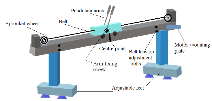
Fig. 1. Digital Pendulum mechanical unit
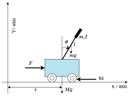
Fig. 2. Cart-Pendulum system
Cart-Pendulum system parameters
| Table 1 | |
|---|---|
| Parameter | Value |
| g - Acceleration due to gravity | 9.81 m/s2 |
| l - Length of the pendulum | 0.4 m |
| M - Mass of the cart | 2.4 kg |
| m - Mass of the pendulum | 0.23 Kg |
| J - Moment of inertia of pendulum | 0.099 Kg.m2 |
| b - Coefficient of cart friction | 0.055 Ns/m |
| d - Pendulum damping coefficient | 0.005 Nm.s/rad |
| F - Applied force to the cart | - 24 N < F < + 24 N |
| x - Position of cart from the reference | - 0.5 m < x < + 0.5 m |
Summing the forces acting on the cart-pendulum system (Fig. 2) the following nonlinear equations of motion are obtained.
$$(m + M) \ddot{x} + b \dot{x} + ml\ddot{\theta} cos\theta - ml\dot{\theta}^2 sin\theta = F \tag{1}$$
$$(I+ml^2)\ddot{\theta} - mglsin\theta + ml\ddot{x}cos\theta + d\dot{\theta} = 0 \tag{2}$$
For such a nonlinear model ((1) and (2)) to be presented as a transfer function, it has to be linearized. For small θ, pendulum damping coefficient (d) and coefficient of cart friction (b) are ignored. Linearization of (1) and (2) can be done by substituting the nonlinear functions (sine and cosine) with their linear equivalent using Taylor approximation of the nonlinear functions. For small angle deviations around an equilibrium point of <span class="fontCss2"style="font-weight:bold">θ = 0 (inverted pendulum) following assumptions can be considered for linearization.
$$sin \theta \approx \theta \tag{3}$$ $$cos \theta \approx 1 \tag{4}$$ $$\dot{\theta}^2 \approx 0 \tag{5}$$
Linearizing (1) and (2), following the assumptions (3), (4), (5) and neglecting d in (2), b in (1), (6) and (7) are obtained.
$$(m + M)\ddot{x} + ml\ddot{\theta} = F \tag{6}$$
$$(I + ml^2)\ddot{\theta} - mgl\theta + ml\ddot{x} = 0 \tag{7}$$
From (6) and (7), (8) and (9) are obtained,
$$\ddot{x} = \frac{1}{\Delta} [(I+ml^2)F - ml(mgl\theta)] \tag{8}$$
$$\ddot{\theta} = \frac{1}{\Delta} [(-ml)F + (m+M)(mgl\theta)] \tag{9}$$
where,
$$\Delta = (I+ml^2)(m+M) - m^2l^2$$
The state vectors are,
$$x_1 = x, \ \ \ x_2 = \dot{x}, \ \ \ x_3 = \theta, \ \ \ x_4 = \dot{\theta}$$
From (8) and (9), the state equations are writen in (10)-(13),
$$\dot{x_1} = x_2 \tag{10}$$
$$\dot{x_2} = \frac{1}{\Delta} [(I+ml^2)F - ml(mgl\theta)] \tag{11}$$
$$\dot{x_3} = x_4 \tag{12}$$
$$\dot{x_4} = \frac{1}{\Delta} [(-ml)F + (m+M)(mgl\theta)] \tag{13}$$
State Space Representation
Utilizing (10)-(13), the state space model is obtained in (14) and (15).
$$\left[\begin{array}{cc}
\dot{x} \newline
\ddot{x}\newline
\dot{\theta}\newline
\ddot{\theta}\newline
\end{array}\right]=\left[\begin{array}{cc}
0 & 1& 0 & 0 \newline
0 & 0 & -\frac{m^2 l^2 g}{\Delta} & 0 \newline
0 & 0& 0 & 1 \newline
0 & 0 & \frac{mgl(m+M)}{\Delta} & 0 \newline
\end{array}\right]
\left[\begin{array}{cc}
x \newline
\dot{x} \newline
\theta \newline
\dot{\theta} \newline
\end{array}\right]+
\left[\begin{array}{cc}
0 \newline
\frac{(I+ml^2)}{\Delta} \newline
0 \newline
\frac{-ml}{\Delta} \newline
\end{array}\right]
F \tag {14}$$
$$y = \ \left[\begin{array}{cc}
1 & 0 & 0 & 0 \newline
0 & 0 & 1 & 0
\end{array}\right]
\left[\begin{array}{cc}
x \newline
\dot{x} \newline
\theta \newline
\dot{\theta} \newline
\end{array}\right] \tag {15}$$
Transfer Function Model
Laplace transform of (7) yields (16).
$$(I + ml^2) s^2 \theta(s) + mls^2 X(s) - mgl \theta(s) = 0$$
$$\Longrightarrow [(I + ml^2) s^2 - mgl] \theta(s) = -mls^2 X(s)$$
$$\frac{X(s)}{\theta(s)} = \frac{-[(I + ml^2) s^2 - mgl]}{mls^2} \tag{16}$$
Considering the value of θ(s) from (16) and substituting it into the Laplace transform of (6), (17) is obtained.
$$(m + M) s^2 X(s) + mls^2 \left(\frac{-mls^2 X(s)}{(I + ml^2)s^2 - mgl}\right) = F(s)$$
$$\Longrightarrow X(s) \left[(M + m) s^2 - \frac{m^2 l^2 s^4}{(I + ml^2) s^2 - mgl}\right] = F(s)$$
$$\Longrightarrow \frac{X(s)}{F(s)} = \frac{(I + ml^2)s^2 -mgl}{(M + m)(I + ml^2) s^4 - (M + m) mgls^2 - m^2l^2s^2} \tag{17}$$
$$m^2l^2 \approx 0 \ (since \ it \ is \ very \ small)$$
$$\Longrightarrow \frac{X(s)}{F(s)} = \frac{(I + ml^2)\left(s^2 - \frac{mgl}{I + ml^2}\right)}{(I + ml^2)(M + m)s^2 \left(s^2 - \frac{mgl}{I + ml^2}\right)}$$
$$\Longrightarrow \frac{X(s)}{F(s)} = \frac{I + ml^2}{(I + ml^2)(M + m) s^2}$$
$$\Longrightarrow \frac{X(s)}{F(s)} = \frac{1}{(M + m) s^2}$$
$$\frac{X(s)}{F(s)} \approx \frac{b_1}{s^2} = P_1 \ where, b_1 = \frac{1}{M + m} \tag{18}$$
Now, substituting the value of X(s) from (16) into the Laplace transform of (6), (19) is obtained,
$$-(M + m) \left[ \frac{ (I + ml^2) s^2 - mgl }{ ml } \theta(s) \right] + mls^2 \theta(s) = F(s)$$
$$\Longrightarrow \frac{\theta(s)}{F(s)} = \frac{ml}{m^2l^2s^2 - (M + m)(I + ml^2)s^2 + (M + m) mgl} \tag{19}$$
We know:
$$\Delta = (M + m)(I + ml^2) - m^2l^2$$
Since m and l are very small, m2l2 will also be small, so it is neglected.
Now,
$$\Delta_1 \approx (M + m)(I + ml^2)$$
$$\Longrightarrow \frac{\theta(s)}{F(s)} = \frac{ml}{-\Delta_1 s^2 + (M + m) mgl}$$
$$\Longrightarrow \frac{\theta(s)}{F(s)} = \frac{ml}{-\Delta_1 [s^2 - \frac{(M + m) mgl}{\Delta_1}]}$$
$$\Longrightarrow \frac{\theta(s)}{F(s)} = \frac{ml}{-\Delta_1 [s^2 - \frac{mgl}{I + ml^2}]}$$
Let,
$$\frac{-ml}{\Delta_1} = b_2 \ and \ \frac{mgl}{I + ml^2} = a_2$$
$$\frac{\theta(s)}{F(s)} = \frac{b_2}{s^2 - a_2} = P_2 \tag{20}$$
Now, the dc motor is used to convert the control voltage U to force F is represented by only a gain block of gain = 15. Hence, after substituting the parameter values from Table 1 into (18) and (20), and multiplying the numerators by a gain of 15, the transfer functions X(s)/U(s) and θ(s)/U(s) are obtained in (21) and (22).
$$\frac{X(s)}{U(s)} \triangleq \frac{b_1}{s^2} = \frac{5.703}{s^2} \tag {21}$$
$$\frac{\theta(s)}{U(s)} \triangleq \frac{b_2}{s^2 - a_2} = \frac{-3.864}{s^2 - 6.646} \tag {22}$$
Two loop PID controller
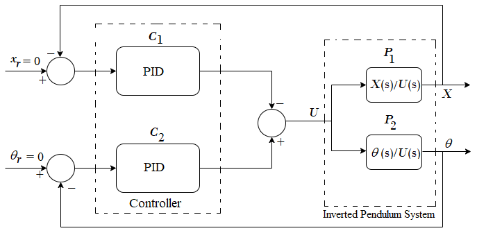
Fig. 3. Two-loop PID controller for an inverted cart–pendulum system
The two-loop PID controller (details in Reference [5]) to be employed for the cart–pendulum system is shown in Fig. 3. Let the two PID controllers be
$$C_1 = \frac{k^1_d s^2 +k^1_p s +k^1_i}{s} \tag {23}$$ $$C_2 = \frac{k^2_d s^2 +k^2_p s +k^2_i}{s} \tag {24}$$
where,
$$k^1_p \ denotes \ proportional \ gain \ for \ C_1$$ $$k^1_i \ denotes \ integral \ gain \ for \ C_1$$ $$k^1_d \ denotes \ derivative \ gain \ for \ C_1$$ $$k^2_p \ denotes \ proportional \ gain \ for \ C_2$$ $$k^2_i \ denotes \ integral \ gain \ for \ C_2$$ $$k^2_d \ denotes \ derivative \ gain \ for \ C_2$$
With the control configuration in Fig. 3, the characteristic equation becomes,
$$1 - P_1C_1 + P_2C_2 = 0 \tag {25}$$
Substituting P1, P2 (from (18) and (20)), and C1, C2 (from (23) and (24)) in (25), we get
$$1 - (\frac{b_1}{s^2}\frac{k^1_d s^2 +k^1_p s +k^1_i}{s})+ (\frac{b_2}{s^2 - a_2}\frac{k^2_d s^2 +k^2_p s +k^2_i}{s}) = 0 \tag {26}$$
which yields
$$s^5 + (-b_1 k^1_d + b_2 k^2_d)s^4 + (-a_2 - b_1 k^1_p + b_2 k^2_p)s^3 + (-b_1 k^1_i + a_2b_1k^1_d + b_2k^2_i)s^2 + (a_2b_1k^1_p)s + (a_2b_1k^1_i) = 0 \tag {27}$$
Since (27) is the characteristic equation of fifth order, let the desired characteristic equation be
$$s^5 + p_1s^4 + p_2s^3 + p_3s^2 + p_4s + p_5 = 0 \tag {28}$$
Comparing the coefficients of (27) and (28), (29) is obtained,
$$\left[\begin{array}{cc}
-b_1 & 0 & 0 & b_2 & 0 & 0 \newline
0 & -b_1 & 0 & 0 & b_2 & 0 \newline
a_2b_1 & 0 & -b_1 & 0 & 0 & b_2\newline
0 & a_2b_1 & 0 & 0 & 0 & 0\newline
0 & 0 & a_2b_1 & 0 & 0 & 0 \newline
\end{array}\right]
\left[\begin{array}{cc}
k^1_d\newline
k^1_p \newline
k^1_i\newline
k^2_d\newline
k^2_p\newline
k^2_i\newline
\end{array}\right]=\left[\begin{array}{cc}
p_1\newline
p_2 + a_2\newline
p_3\newline
p_4\newline
p_5\newline
\end{array}\right]
\tag {29}$$
LQR Design
The LQR is an optimal state feedback controller designed to minimise a particular quadratic performance index, which takes care of the design constraints. For an LTI system,$$\dot{X}= AX + BU$$ $$Y=CX \tag {30}$$
The performance index is taken as, $$J = \frac{1}{2}\int_{0}^{\infty} (X^TQX + U^TRU) dt \tag {31}$$
where, Q is positive semi-definite (or positive definite) and R is positive definite. The minimisation of J is obtained by solving the algebraic Riccati equation –
$$A^TP+PA-PBR^{-1}B^TP+Q = 0 \tag {32}$$ The optimal state feedback gain vector K ≜ [K1, K2, K3, K4] becomes,
$$K = -R^{-1}B^TP \tag {33}$$
Now for the inverted pendulum system (presented in (14) and (15)), the LQR design is carried out. By substituting the system parameter values from Table 1 into (14) and (15), and then comparing these equations with (30), we obtain
$$A =\left[\begin{array}{cc}
0 & 1 & 0 & 0\newline
0 & 0 & -0.238 & 0 \newline
0 & 0 & 0 & 1\newline
0 & 0 & 6.807 & 0\newline
\end{array}\right],
B =\left[\begin{array}{cc}
0\newline
0.3894\newline
0\newline
-0.2638\newline
\end{array}\right]\times 15,
\ C =\left[\begin{array}{cc}
1 & 0 & 0 & 0\newline
0 & 0 & 1 & 0 \newline
\end{array}\right]
\tag {34}$$
The Q matrix and R are taken as,
$$Q =\left[\begin{array}{cc} 50000 & 0 & 0 & 0\newline 0 & 2000 & 0 & 0 \newline 0 & 0 & 2000 & 0 \newline 0 & 0 & 0 & 100 \newline \end{array}\right], R = 10000$$
The optimal state feedback control gains are then found to be,
$$K = [-2.2361 \ -2.7209 \ -17.5208 \ -6.7791]^T \tag {35}$$
Finally, the closed-loop poles, i.e., the eigen-values of (A – BK) are obtained as -2.8862 ± 2.1606 i, -2.58 ± 0.1461 i
Now, with four closed-loop poles and choosing the fifth pole to be six times the real part of the
dominant one among these four poles, the coefficients of (28) are obtained as, p1= 26.4, p2= 218.6, p3= 871.3, p4= 1721.8, p5= 1343.7.
Next, by substituting these p1, p2, p3, p4, p5 and b1, b2, a2 obtained from (21), (22) in (29), we get
$$\left[\begin{array}{cc}
-5.703 & 0 & 0 & -3.863 & 0 & 0\newline
0 & -5.703 & 0 & 0 & -3.863 & 0\newline
37.9021 & 0 & -5.703 & 0 & 0 & -3.863\newline
0 & 37.9021 & 0 & 0 & 0 & 0\newline
0 & 0 & 37.9021 & 0 & 0 & 0\newline
\end{array}\right]
\left[\begin{array}{cc}
k^1_d\newline
k^1_p \newline
k^1_i\newline
k^2_d\newline
k^2_p\newline
k^2_i\newline
\end{array}\right]=\left[\begin{array}{cc}
26.4\newline
225.25\newline
871.3\newline
1721.8\newline
1343.7\newline
\end{array}\right]
\tag {36}$$
In (36), five poles need to be placed and we have six parameters. So we need to fix one parameter.
On choosing kd2 = 10 (say), the PID parameters are obtained as
$$k^1_p =45.429 $$
$$k^1_d =-11.403 $$
$$k^1_i =35.453 $$
$$k^2_p =-125.442 $$
$$k^2_i = -389.786$$
Application
- The Segway
- The human posture systems
- The launching of a rocket etc.
Observations :
- It has been observed that the derived controller works for real time plant for an initial angle approximately -6° (≈-0.1 rad) ≤ θ ≤ +6° (≈+0.1 rad).
- For an initial angle -6° (≈-0.1 rad) > θ or θ > +6° (≈+0.1 rad) the real time plant becomes unstable as the controller doesnot get activated, i.e., the initial angle value comes under unstable zone.
- The experiment has been developed based on pure mathematical modelling. In practical case, results may defer due to some additional environmental or physical factors.
Integral Square Error (ISE): In control system engineering, performance indices (PP-182 (Reference [3]), PP-654 (Reference [4])) are critical in evaluating the effectiveness of controller parameters. One of the most widely used performance indices is ISE. It provides a quantitative measure of how well a system tracks a reference signal. ISE is defined as the integral of square of the error signal over a specified time interval T. Mathematically, the integral computes the area under the curve of squared error over time and it is denoted in (37).
$$ISE = \int_{0}^{T} e^2 (t) dt \tag{37}$$
where,
- e(t) - error between reference signal r(t) and actual output y(t).
- T - total simulation time.
- e2(t) - square of error at t th time instant.
Utilization of ISE in Inverted Cart-Pendulum
In the context of the inverted cart-pendulum system,
In (38), ISE represents a quantitative measure of how much the pendulum angle deviates from its vertical upright (zero-angle) position over time T.
$$ISE = \int_{0}^{T} e_{\theta}^2 (t) dt \tag{38}$$
A lower value of ISE indicates superior controller performance.
Effect of changing kd2 on other gains and ISE values
| Table 2 | ||||
|---|---|---|---|---|
| Initial angle (°) | kd2 | kd1 | ki2 | ISE |
| 6 | 10 | -11.403 | -389.768 | 0.012937 |
| 6 | 20 | -18.176 | -456.220 | 130.36807 |
Conclusion :
Table 2 data reveals that,
- The value of kd2 must be a positive integer, i.e. kd2 ∈ Z+ where, Z+ denotes the set of positive integers.
- A moderate value of kd2 (say 10) provides a good system performance.
- A high values of kd2 (say 20) lead to poor system performance, as indicated by high ISE value.