Introduction

Uniform Cost Search (UCS) is an uninformed search algorithm for traversing a graph. UCS evaluates and explores nodes by considering the cost to reach the node (g). The algorithm selects the node with the lowest g value to explore next. We typically use a priority queue (frontier) to select the node with the lowest g value for expansion. It is a fundamental algorithm used in various applications such as pathfinding, robotics, route planning, and optimization problems due to its completeness, optimality, and optimal efficiency.

Algorithm

The UCS Search algorithm is a pathfinding algorithm used to find the shortest path from a start node to a goal node in a graph with edge weights, taking into account the actual cost from the start node to the node. The cost function g(n) gives the actual cost to reach node n from the start node and is what the priority queue is ordered by.

STEP 1: Initialize the frontier (priority queue) with the start node 'start' and set the path cost g(start) to 0.

STEP 2: Initialize an empty set "visited" to keep track of the explored nodes.

STEP 3: While the frontier is not empty, select the node with the lowest path cost value (g), which represents the least-cost node.

STEP 4: If the selected node is the goal node, reconstruct and return the path from the start node to the goal node.

STEP 5: If the selected node is not the goal node, remove the node from the frontier and add it to the explored set. Expand the selected node by exploring its neighbors and update the cost and parent of each neighbor.

STEP 6: For each neighbor, if it is not already in the visited set, calculate the tentative g value, update it if it is lower than the current g value, and add it to the frontier.

STEP 7: Repeat steps 3-6 until the goal node is reached or the frontier is empty.

Example

Reference: Section 3.4.2 of Reference 1

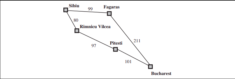
The task is to navigate from Sibiu to Bucharest using a uniform-cost search. From Sibiu, the connected nodes are Rimnicu Vilcea and Fagaras, with travel costs of 80 and 99, respectively. Since Rimnicu Vilcea has the lower cost, it is explored first. Expanding Rimnicu Vilcea reveals a path to Pitesti with a cumulative cost of 80+97=177.

Next, Fagaras, which is now the least-cost node, is explored. This expansion leads to Bucharest with a total cost of 99+211=310. Although the goal node Bucharest has been reached, since it has not been selected for expansion, the algorithm continues, prioritizing Pitesti for expansion due to its lower cumulative cost. This results in an alternative route to Bucharest via Pitesti, with a total cost of 80+97+101=278.

Now the algorithm checks to see if this new path is better than the old one; it is, so the old one is discarded.Finally, Bucharest is selected for expansion with the updated cost of 278, and the solution is returned.

Optimality and Completeness

Optimality: UCS is optimal for non-negative edge costs. Whenever UCS selects a node n for expansion, the optimal path to that node has been found. If there exists a better path to node n, it must have passed through some other frontier node n' before reaching node n. By definition, node n' would have lower g-cost than n and would have been selected first. Therefore, if UCS selects n for expansion, it has evaluated and discarded any potential paths to n that are not optimal.

Completeness: UCS does not care about the number of steps a path has, but only about their total cost. It will get stuck in an infinite loop if there is a path with an infinite sequence of zero cost actions. Completeness if guaranteed provided the cost of every step exceeds some small positive constant $\epsilon$.

Space and Time Complexity

Let $b$ be the branching factor of the graph. Let $C*$ be the cost of the optimal solution and assume that every action costs at least $\epsilon$. Then the algorithm's worst time and space complexity is $O(b^{1 + \lfloor C^*/\epsilon \rfloor})$. This is because in the worst case, the optimal path is a series of small steps where each step size is the minimum possible value ($\epsilon$). When all step costs are equal, $b^{1 + \lfloor C^*/\epsilon \rfloor}$ becomes $b^{1+d}$ where d is the depth of the goal node. This is similar to breadth first search, except that the latter stops as soon as it generates a goal node, whereas UCS stops when it selects the goal node for expansion.

Advantages

Optimality: UCS guaranteed finding the optimal solution in terms of cost, provided that the step costs are non-negative.

Completeness: UCS is complete, meaning it will always find a solution if one exists, as long as the step costs are greater than some small positive constant.

Flexibility: UCS can handle graphs with varying edge costs and does not require any assumptions about the structure of the graph other than non-negative edge costs. This makes it suitable for a wide range of problems.

Disadvantages

Time Complexity: UCS can have a high time complexity, especially when dealing with graphs with high branching factors or when the optimal solution is deep in the search tree. Its time complexity is very high in cases where UCS explores large trees of small steps before exploring paths involving large and perhaps useful steps.

Space Complextiy: UCS requires storing all explored nodes in memory to determine the optimal path. In scenarios with large graphs or limited memory resources, this can become a significant drawback, as the memory usage increases with the size of the search space.

Sensitivity to Edge Costs: UCS assumes that the step costs between nodes are non-negative. If there are negative edge costs or if the cost of reaching a node changes dynamically during the search, UCS may not guarantee optimal results.

Inefficiency with Uniform Costs: While UCS excels in finding optimal solutions when step costs vary, it can be inefficient in scenarios where all step costs are uniform. In such cases, other search algorithms like Breadth First Search may perform better.

Lack of Heuristic Information: UCS does not utilize any heuristic information about the problem domain. While this ensures optimality, it may lead to suboptimal performance in domains where heuristic information can guide the search more efficiently, such as in informed search algorithms like A*.