
Types of Oscillators: Simple Harmonic, Damped and Forced Oscillators
Procedure for the experiment is as follows:
1. To study Simple Harmonic Motion
Step 1: Set the damping factor (b) = 0.
Step 2: Set v0 = 0 m/s.
Step 3: Drag the ball to the maximum starting position, say x0 = 10.0 m, and click the play animation button.
Step 4: Observe the position graph as shown in Fig. 1 and wait until the animation ends.
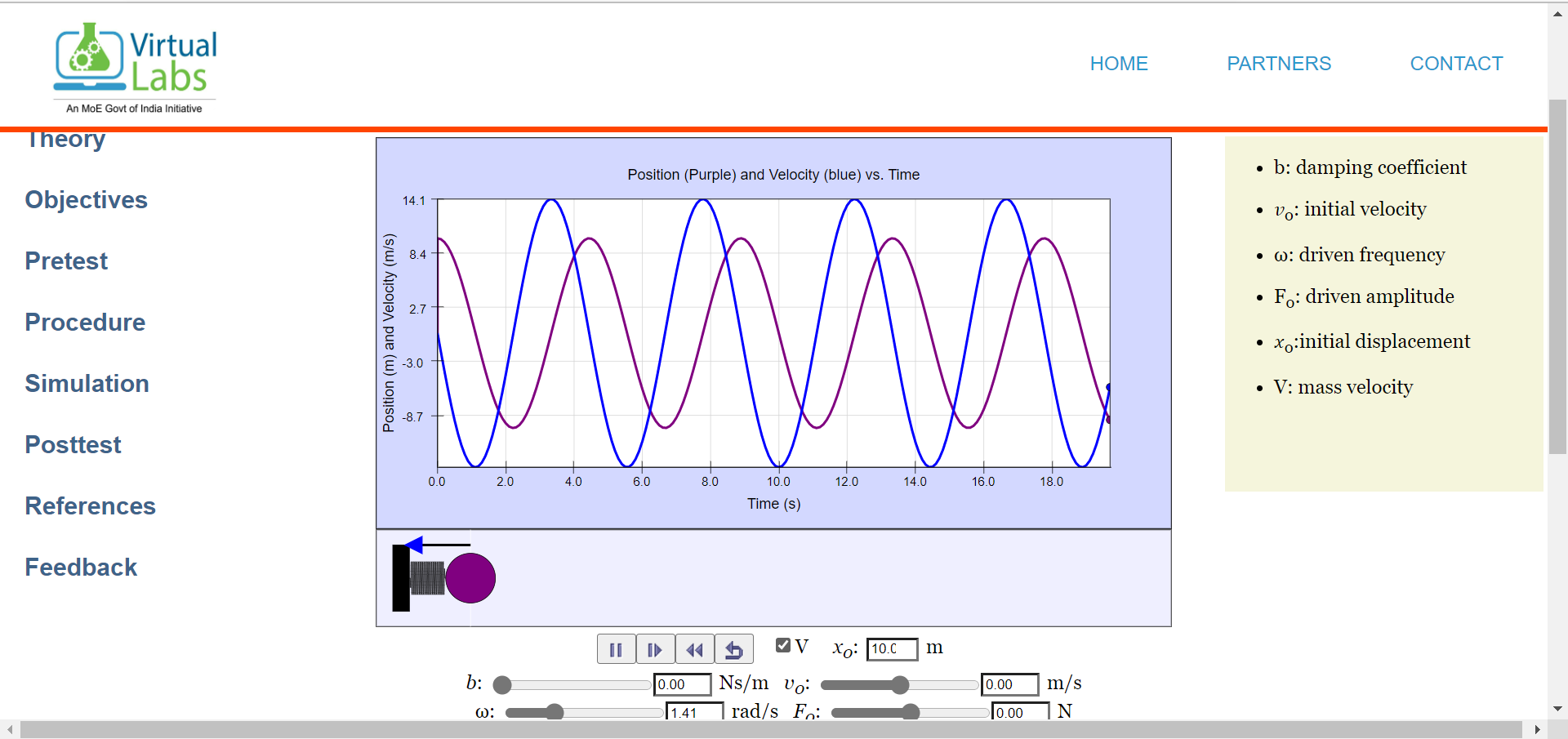
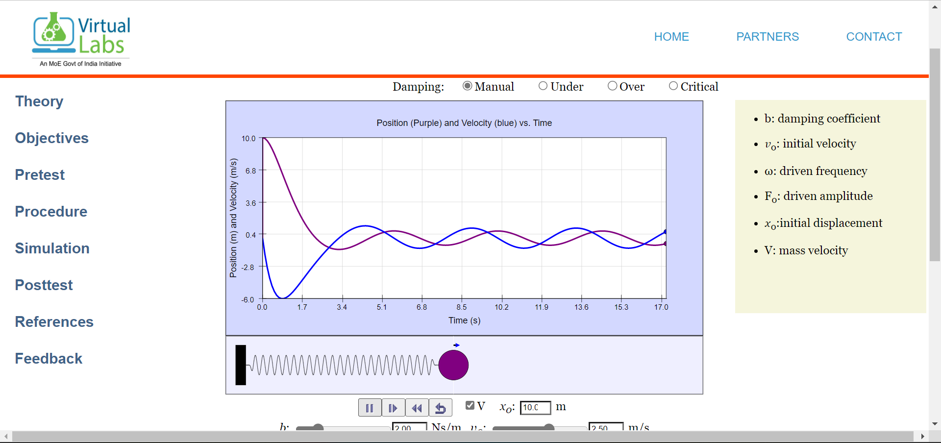
Step 5: To get the position and velocity graph as shown in Fig. 2, tick the velocity checkbox (V).
Fig. 1: Graph representing S.H.M. motion (position vs time)
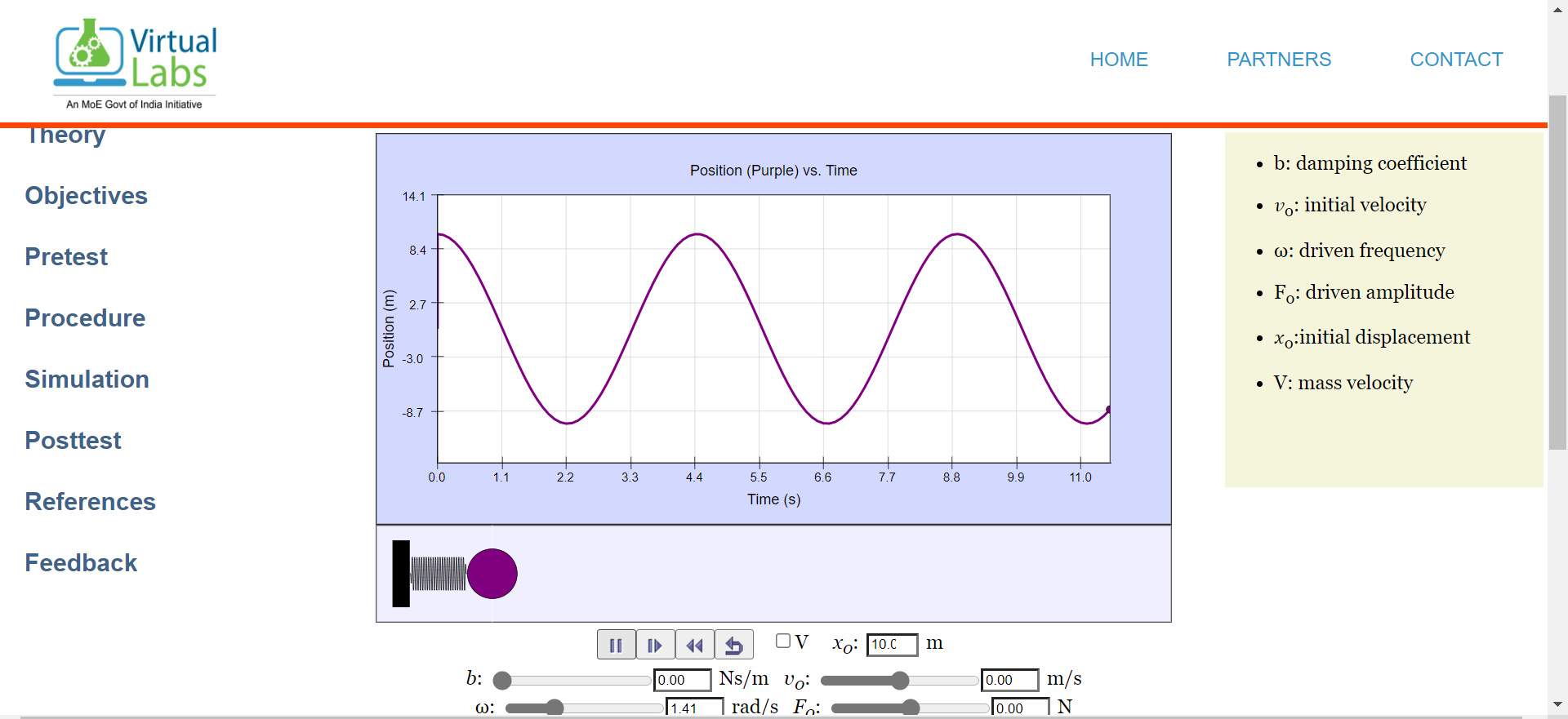
Fig. 2: Graph representing S.H.M. motion (position and velocity vs time)
2. To study Damped Oscillatory Motion
Step 1: Reset the simulation.
Step 2: Set v0 = 0 m/sec.
Step 3: Change the damping factor (b) (for example, b = 0.5, 2.83 or 3).
Step 4: Drag the ball to the maximum initial position, say x0 = 10.0 m and click the play button.
Step 5: Perform the experiment for three different values of the damping factor (b = 0.5, 2.83 and 3), resetting the simulation for each case.
Step 6: Repeat the entire procedure as done previously.
Note: After selecting any damping checkbox (Under, Over, or Critical), the value of b is automatically set — no need to manually enter it.
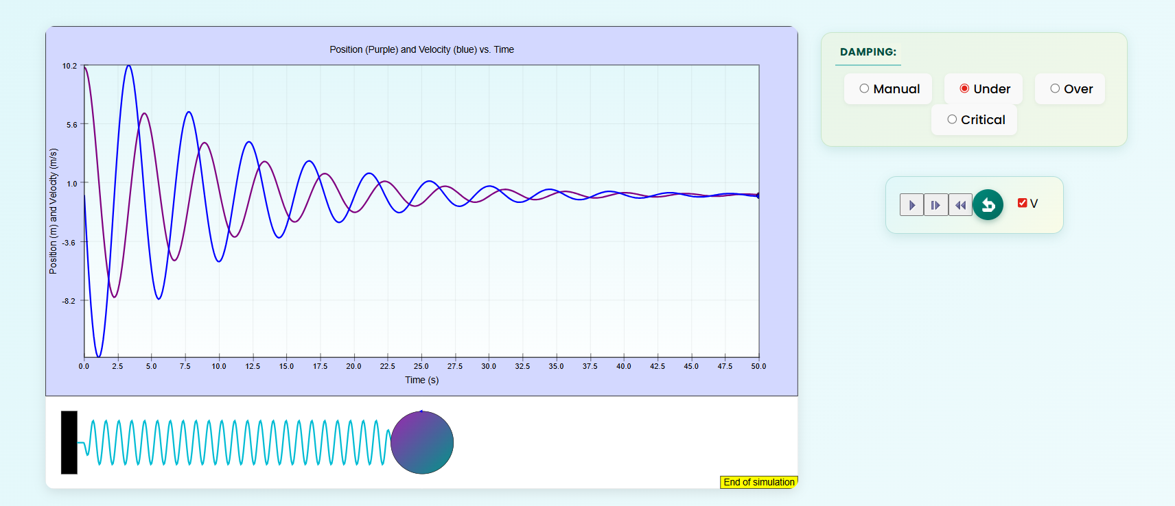
Case 1: Under-Damping
Case 2: Critical-Damping
Case 3: Over-Damping
Set the value of b < 2√2 (say b = 0.5)
Fig. 3: Graph representing under-damped oscillatory motion (position vs time)
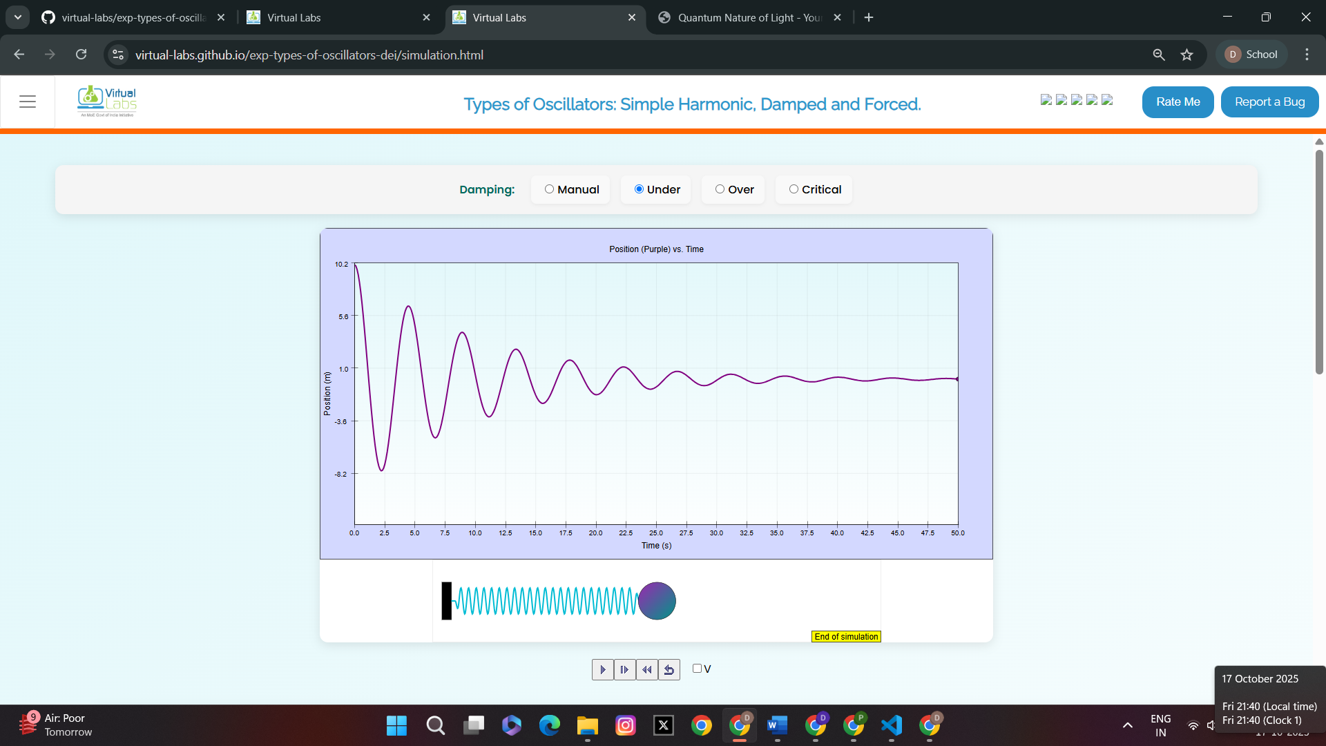
Fig. 4: Graph representing under-damped oscillatory motion (position and velocity vs time)
Set the value of b = 2√2 ≈ 2.83
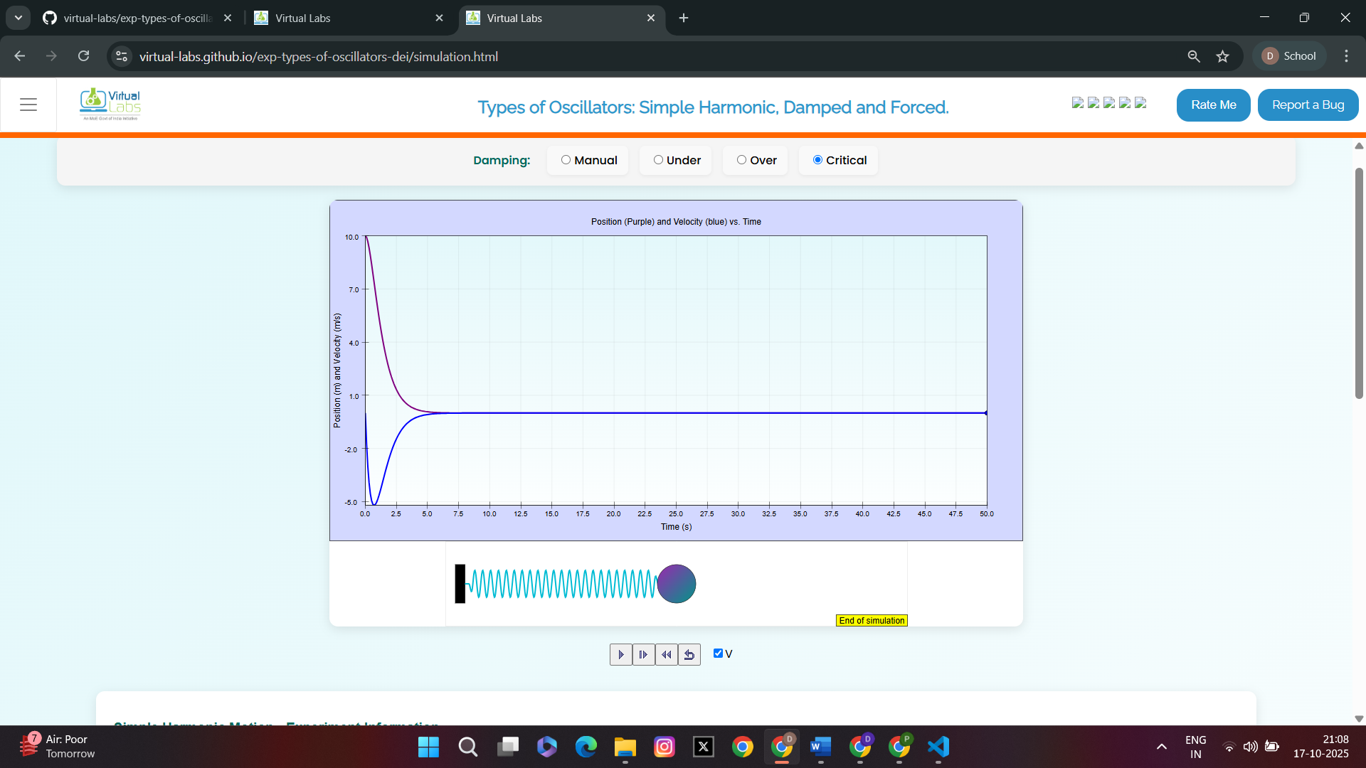
Fig. 5: Graph representing critically-damped oscillatory motion (position vs time)
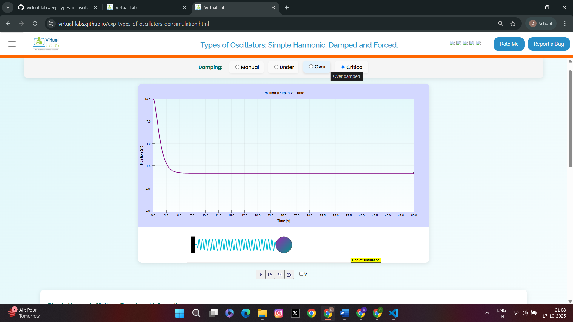
Fig. 6: Graph representing critically-damped oscillatory motion (position and velocity vs time)
Set the value of b > 2√2 (say b = 3)
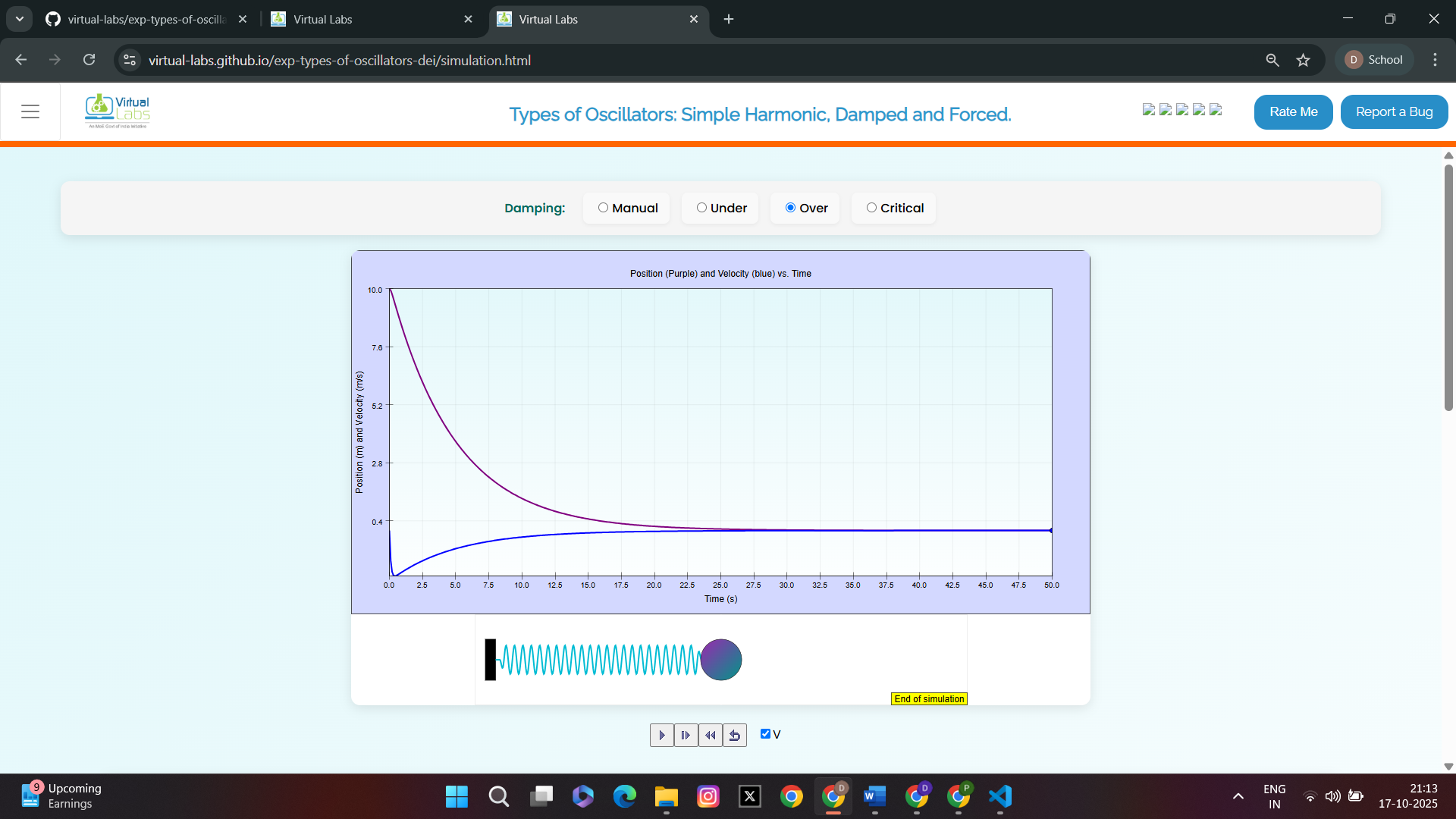
Fig. 7: Graph representing over-damped oscillatory motion (position vs time)

Fig. 8: Graph representing over-damped oscillatory motion (position and velocity vs time)
In all the above cases, observe the graph and wait until the animation ends.
3. To study Forced Oscillatory Motion
Step 1: Reset the simulation again.
Step 2: Set the damping coefficient (b) > 2√2 (say b = 3).
Step 3: Change the value of initial velocity v0 = 2 m/sec.
Step 4: Set value of driven angular frequency (ω) = 1.41 rad/s.
Step 5: Set some value of driven amplitude F0 which will be the force for oscillation.
Step 6: Drag the ball to the maximum starting position, say x0 = 10.0 m and press the play button.
Step 7: Observe the graph till the animation ends.
Fig. 9: Graph representing forced-oscillatory motion (position vs time)
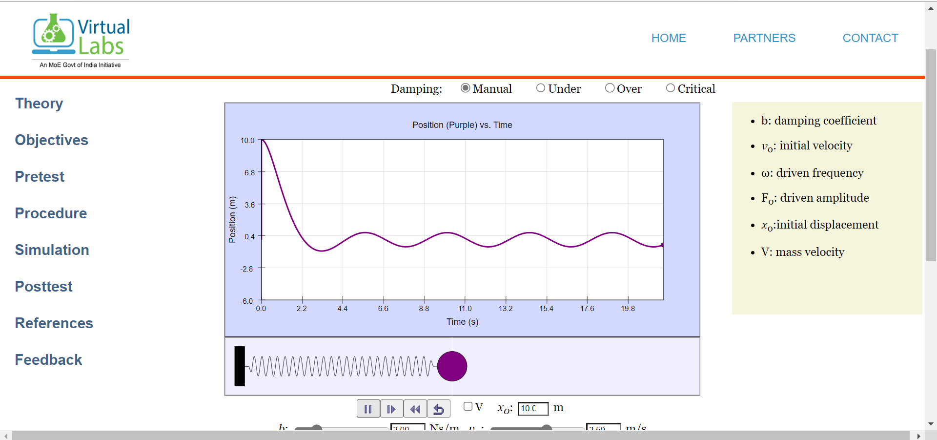
Fig. 10: Graph representing forced-oscillatory motion (position and velocity vs time)
Perform the following experiments
Experiment 1:
Perform an experiment to calculate the value of k (spring constant) for the cases described below. In each case, record the observations in the table and compute the value of k. Take the value of m = 1 kg in each case.
Case 1: Free oscillator (Simple Harmonic Motion) when b = 0
Set different values for x0.
Keep other parameters = 0.
Record the value of time period (T) in each case.
Calculate the corresponding angular frequency ω = 2π/T.
Then compute k (spring constant) using the formula:

ω = √(k/m) ⇒ k = mω²
Table 1: Test values for Free Oscillator (b = 0, v0 = 0, m = 1 kg)
| S.No | x0 (m) | T (s) | f (Hz) | ω (rad/s) |
|---|---|---|---|---|
| 1 | 1.0 | 4.44 | 0.225 | 1.414 |
| 2 | 2.0 | 4.44 | 0.225 | 1.414 |
| 3 | 4.0 | 4.44 | 0.225 | 1.414 |
| 4 | 6.0 | 4.44 | 0.225 | 1.414 |
| 5 | 8.0 | 4.44 | 0.225 | 1.414 |
| 6 | 10.0 | 4.44 | 0.225 | 1.414 |
The mean ω = 1.414 rad/s
Computed value of k = mω² = 1 × (1.414)² = 2.0 N/m
Case 2: Under-Damped Oscillator when b < 2√2 (say b = 0.5)
Set different values for x0.
Set b = 0.5 Ns/m and keep other parameters = 0.
Record the value of time period (T) in each case.
Calculate the corresponding damped angular frequency:
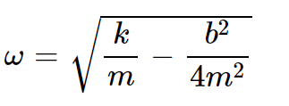
ωd = √(k/m − b²/(4m²))
Value of b used in the experiment: 0.5 Ns/m
Table 2: Test values for Under-Damped Oscillator (b = 0.5, v0 = 0, m = 1 kg)
| S.No | x0 (m) | T (s) | f (Hz) | ωd (rad/s) |
|---|---|---|---|---|
| 1 | 1.0 | 4.51 | 0.222 | 1.392 |
| 2 | 2.0 | 4.51 | 0.222 | 1.392 |
| 3 | 4.0 | 4.51 | 0.222 | 1.392 |
| 4 | 6.0 | 4.51 | 0.222 | 1.392 |
| 5 | 8.0 | 4.51 | 0.222 | 1.392 |
| 6 | 10.0 | 4.51 | 0.222 | 1.392 |
The mean ωd = 1.392 rad/s
Computed value of k = m(ωd² + b²/(4m²)) = 1 × (1.9375 + 0.0625) = 2.0 N/m
Case 3: Forced oscillator when b > 2√2 (say b = 3)
Set different values for F0.
Set driven angular frequency ω = 1.41 rad/s.
Obtain the value of steady-state amplitude (A) by observing the graph each time.
Obtain the value of natural frequency ω0 using the relation:
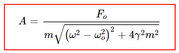
A = F0 / √((k − mω²)² + b²ω²)Then compute k (spring constant) from the calculated mean value of ω0.
Parameters: b = 3 Ns/m, ωdrive = 1.41 rad/s, x0 = 10 m, v0 = 2 m/s
Table 3: Test values for Forced Oscillator (b = 3, ω = 1.41 rad/s, m = 1 kg)
| S.No | F0 (N) | A (m) | ω0 (rad/s) |
|---|---|---|---|
| 1 | 1.0 | 0.236 | 1.414 |
| 2 | 2.0 | 0.473 | 1.414 |
| 3 | 3.0 | 0.709 | 1.414 |
| 4 | 5.0 | 1.182 | 1.414 |
| 5 | 8.0 | 1.891 | 1.414 |
| 6 | 10.0 | 2.364 | 1.414 |
The mean ω0 = 1.414 rad/s
Computed value of k = mω0² = 1 × (1.414)² = 2.0 N/m