Automotive Vehicle as a Two Degree of Freedom System
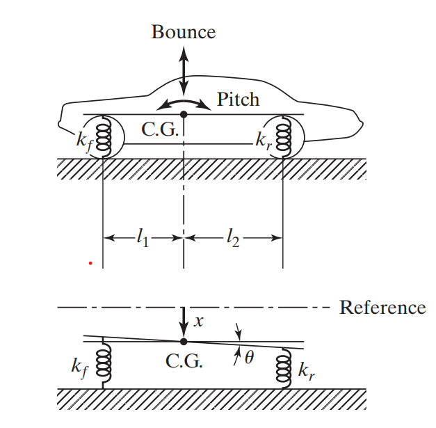
An automobile carries passengers or goods from one place to another. Generally, it consists of a suspension, tire, and other electrical systems which assist in either the maintenance or efficient functioning of the vehicle. The automobile can be modeled as a two-degree-of-freedom lumped parametric system to study pitch and bounce motions, as shown in Figure 1.
Fig. 1. Pitch and bounce motion of a Car
As a two-degree of freedom system, x (bounce) and θ (pitch) are the independent parameters that will give the equations of motion.
m x ¨ = − k f ( x − l 1 θ ) − k r ( x + l 2 θ ) m\ddot x = -k_f(x - l_1 \theta) - k_r(x+l_2\theta) m x ¨ = − k f ( x − l 1 θ ) − k r ( x + l 2 θ )
J 0 θ ¨ = k f ( x − l 1 θ ) l 1 − k r ( x + l 2 θ ) l 2 J_0\ddot \theta = k_f(x - l_1 \theta)l_1 - k_r(x + l_2\theta)l_2 J 0 θ ¨ = k f ( x − l 1 θ ) l 1 − k r ( x + l 2 θ ) l 2
In the matrix form,
[ m 0 0 J 0 ] { x ¨ θ ¨ } + [ ( k f + k r ) − ( k f l 1 − k r l 2 ) − ( k f l 1 − k r l 2 ) ( k f l 1 2 + k r l 2 2 ) ] { x θ } = { 0 0 }
\begin{bmatrix}
m & 0 \\
0 & J_{0}
\end{bmatrix}
\begin{Bmatrix}
\ddot{x} \\
\ddot{\theta}
\end{Bmatrix} +
\begin{bmatrix}
(k_{f} + k_{r}) & -(k_{f}l_{1} - k_{r}l_{2}) \\
-(k_{f}l_{1} - k_{r}l_{2}) & (k_{f}l_{1}^{2} + k_{r}l_{2}^{2})
\end{bmatrix}
\begin{Bmatrix}
x \\
\theta
\end{Bmatrix} =
\begin{Bmatrix}
0 \\
0
\end{Bmatrix}
[ m 0 0 J 0 ] { x ¨ θ ¨ } + [ ( k f + k r ) − ( k f l 1 − k r l 2 ) − ( k f l 1 − k r l 2 ) ( k f l 1 2 + k r l 2 2 ) ] { x θ } = { 0 0 }
Assuming a harmonic solution,
x ( t ) = X c o s ( ω t + ϕ ) θ ( t ) = θ cos ( ω t + ϕ ) x(t) = X cos(\omega t + \phi) \space \space\space\space\space\space\space\space\space\space\space\space\space \theta(t) = \theta \cos(\omega t + \phi) x ( t ) = X cos ( ω t + ϕ ) θ ( t ) = θ cos ( ω t + ϕ )
We get,
[ ( − m ω 2 + k f + k r ) ( − k f l 1 + k r l 2 ) ( − k f l 1 + k r l 2 ) ( − J 0 ω 2 + k f l 1 2 + k r l 2 2 ) ] { X θ } = { 0 0 }
\begin{bmatrix}
(-m\omega^{2}+k_{f}+k_{r}) & (-k_{f}l_{1}+k_{r}l_{2}) \\
(-k_{f}l_{1}+k_{r}l_{2}) & (-J_{0}\omega^{2}+k_{f}l_{1}^{2}+k_{r}l_{2}^{2})
\end{bmatrix}
\begin{Bmatrix}
X \\
\theta
\end{Bmatrix}
=
\begin{Bmatrix}
0 \\
0
\end{Bmatrix}
[ ( − m ω 2 + k f + k r ) ( − k f l 1 + k r l 2 ) ( − k f l 1 + k r l 2 ) ( − J 0 ω 2 + k f l 1 2 + k r l 2 2 ) ] { X θ } = { 0 0 }
Upon solving and simplifying,
J 0 m ω 4 − [ ( k f l 1 2 + k r l 2 2 ) m + ( k f + k r ) I 0 ] ω 2 + K f K r L 2 = 0 J_{0}m\omega^{4}-[(k_{f}l_{1}^{2}+k_{r}l_{2}^{2})m+(k_{f}+k_{r})I_{0}]\omega^{2}+K_{f}K_{r}L^{2}=0 J 0 m ω 4 − [( k f l 1 2 + k r l 2 2 ) m + ( k f + k r ) I 0 ] ω 2 + K f K r L 2 = 0
Where L = l 1 + l 2 L = l_1 + l_2 L = l 1 + l 2
This equation is used to solve for ω, which are the roots of the equation
ω 1 , 2 2 = [ ( k f l 1 2 + k r l 2 2 ) m + ( k f + k r ) I 0 ] ± [ ( k f l 1 2 + k r l 2 2 ) m + ( k f + k r ) I 0 ] 2 − [ 4 I 0 m K f K r L 2 ] 2 I 0 m \omega^{2}_{1,2}=\frac{[(k_{f}l_{1}^{2} \space + \space k_{r}l_{2}^{2}) m\space + \space(k_{f}+k_{r})I_{0}]\space\pm\space\sqrt{[(k_{f}l_{1}^{2}\space +\space k_{r}l_{2}^{2})m\space+\space(k_{f}\space +\space k_{r})I_{0}]^{2}\space -\space [4I_{0}mK_{f}K_{r}L^{2}}]}{2I_{0}m} ω 1 , 2 2 = 2 I 0 m [( k f l 1 2 + k r l 2 2 ) m + ( k f + k r ) I 0 ] ± [( k f l 1 2 + k r l 2 2 ) m + ( k f + k r ) I 0 ] 2 − [ 4 I 0 m K f K r L 2 ]