1. Introduction

The Fibonacci series is one of the most famous numerical sequences in mathematics and computer science.
It appears in many real-world applications such as algorithm design, data structures, nature patterns, and problem-solving techniques.

In programming, the Fibonacci series is commonly used to understand:

• Looping concepts
• Function calls
• Recursion
• Time and space complexity comparison

Real-World Applications

• Used in algorithm analysis to explain recursion and dynamic programming
• Applied in data structures like trees and heaps
• Seen in nature patterns such as leaf arrangement and shell spirals
• Used in financial models for trend and ratio analysis
• Helpful in teaching problem-solving and optimization techniques

---

2. Definition of Fibonacci Series

The Fibonacci series is a sequence of numbers where each number is the sum of the previous two numbers.

Mathematical Definition:

• F(0) = 0
• F(1) = 1
• F(n) = F(n−1) + F(n−2) for n ≥ 2

Example:

0, 1, 1, 2, 3, 5, 8, 13, 21, ...

---

3. Methods to Generate Fibonacci Series

There are two commonly used programming approaches:

1. Iterative Method
2. Recursive Method

Each approach has its own advantages and disadvantages.

Dynamic programming bridges these two approaches by combining recursive problem decomposition with iterative-style reuse of previously computed results (memoization/tabulation).

---

4. Iterative Approach

Concept

The iterative approach generates the Fibonacci series using loops such as for or while.
It calculates each Fibonacci number step-by-step and stores only the required values.

Working Principle

• Initialize the first two numbers
• Use a loop to calculate the next terms
• Update values in each iteration

Pseudocode

          FibonacciIterative(n):
            if n == 0:
              return 0
            if n == 1:
              return 1
          
          a ← 0  
          b ← 1  
          
          for i ← 2 to n do  
             c ← a + b  
             a ← b  
             b ← c  
          end for
          
          return b   // nth Fibonacci number
          
          

Flowchart: Iterative Fibonacci

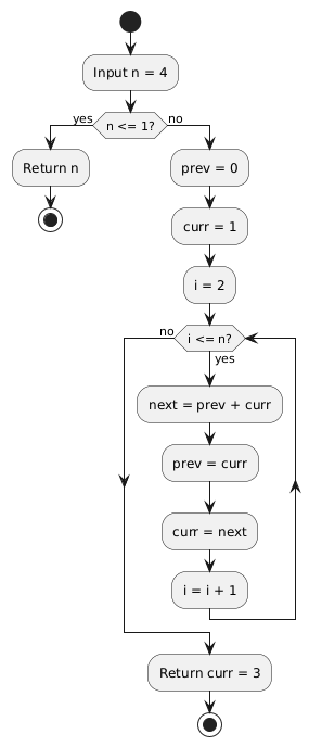
The flowchart illustrates the iterative process for finding 4th Fibonacci number.

Advantages

• Faster execution time
• Uses less memory
• Simple and efficient for large values of n

Disadvantages

• Logic may look less mathematical compared to recursion

---

5. Recursive Approach

Concept

The recursive approach uses function calls where a function calls itself to calculate Fibonacci numbers.

Working Principle

• The recursion stops at base cases (n = 0 and n = 1)
• For other values, the function calls itself to compute the two previous Fibonacci numbers
• The final value is obtained by adding results of smaller subproblems

Pseudocode

          F(n):
            if n == 0:
                return 0
            if n == 1:
                return 1
            return F(n-1) + F(n-2)
          

Recursion Tree: Recursive Fibonacci

F(4)
          ├── F(3)
          │   ├── F(2)
          │   │   ├── F(1) = 1
          │   │   └── F(0) = 0
          │   └── F(1) = 1
          └── F(2)
            ├── F(1) = 1
            └── F(0) = 0
          

The recursion tree for F(4) shows repeated subproblems (for example, F(2) is computed multiple times), which causes inefficiency in naive recursion.

Advantages

• Simple and close to mathematical definition
• Easy to understand conceptually

Disadvantages

• Slower execution time due to repeated calculations
• Uses more memory space (stack calls)
• Inefficient for large values of n

---

6. Comparison: Iterative vs Recursive

Feature	Iterative Approach	Recursive Approach
Execution Speed	Fast – computes each term once in a single pass	Slow – recalculates the same subproblems multiple times
Time Complexity	O(n) – linear growth with input size	Θ(φⁿ) where φ ≈ 1.618 – exponential growth due to overlapping subproblems
Space Complexity	O(1) – uses only a fixed number of variables	O(n) – requires stack space proportional to recursion depth
Memory Usage	Low – no additional stack frames needed	High – each recursive call adds a new frame to the call stack
Risk of Integer Overflow	Present for very large n with fixed-size integer types	Present for very large n with fixed-size integer types
Risk of Stack Overflow	None – no recursion involved	High – deep recursion for large n can exceed stack limit
Scalability	Highly scalable for large values of n	Not scalable – becomes impractical for n > 30–40
Function Call Overhead	None – all computation happens within a single function	Significant – each call incurs overhead for stack management
Suitability for Optimization	Already optimal for basic Fibonacci	Can be optimized using memoization or dynamic programming
Best Use Case	Production code, large inputs, performance-critical applications	Teaching recursion concepts, small inputs, algorithm demonstrations

Key Insights

• For practical applications, the iterative method is almost always preferred due to its efficiency and predictable performance.
• For educational purposes, the recursive method helps students understand the concept of breaking problems into smaller subproblems.
• Dynamic programming acts as a bridge between recursion and iteration: memoization preserves recursive thinking, while tabulation follows an iterative build-up.
• Optimization techniques like memoization can improve recursive performance to O(n), though recursive memoization may still carry stack overhead compared to pure iteration.

---

7. Time and Space Complexity

Iterative Method

• Time Complexity: O(n)
  The loop runs once for each value from 0 to n, performing a constant amount of work each time.
• Space Complexity: O(1)
  Only a few variables are used, regardless of the value of n.

Recursive Method (Naive)

• Time Complexity: Θ(φⁿ) where φ = (1 + √5)/2 ≈ 1.618
  The number of recursive calls grows exponentially and is more tightly bounded by powers of the golden ratio than by 2ⁿ.
• Space Complexity: O(n)
  The maximum recursion depth is n, so the call stack grows linearly with n.

Practical Limitation: Integer Overflow

• With fixed-width integer types (for example, 32-bit or 64-bit), values eventually exceed the maximum representable limit.
• For large n, use big integer libraries/types (such as BigInt) to avoid overflow.

---

8. Conclusion

Both iterative and recursive methods are important for learning programming concepts.

• Iterative approach is preferred for performance and real-world applications.
• Recursive approach is useful for understanding recursion and mathematical problem-solving.

Understanding both methods helps students choose the right approach based on the problem requirements.

For further reading, refer to: Fibonacci and Recurrences (Cornell CS2110)

---