
Study of Rectilinear Motion 
Theory
Rectilinear Motion
Rectilinear motion is another name of straight-line motion. This type of motion describes the movement of a particle or a body.
A body is said to experience rectilinear motion if any two particles of the body travel the same distance along two parallel straight lines.
The fig 1 illustrates rectilinear motion for a body.
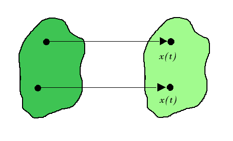
Fig. 1. Rectilinear Motion
The experimental control system in practical laboratory is comprised of the electromechanical plant which consists of the spring-mass mechanism, its actuator and sensors and a subsystem
i.e. an operating program or software which runs on a PC .
Encoder
An encoder is a sensor that converts a positional output into an electronic signal. In this experiment, encoder counts are used as the system units of position, where the counts correspond to the encoder pulses and controller-internal register values. Here, 1 encoder revolution is equivalent to 16,000 encoder counts, which corresponds to 7.06 cm.
Rectilinear Motion Setup in Control Systems
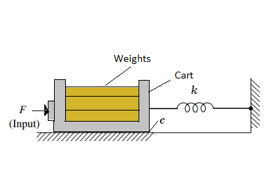
Fig. 2. Rectilinear Motion Setup without dashpot connected
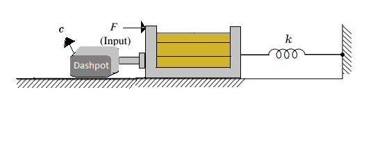
Fig. 3. Rectilinear Motion Setup with dashpot connected
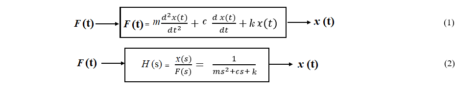
Re arranging the equation (2) and comparing the denominator terms with the characteristics equation of a second order control system we get,
$$s^2 + 2 \zeta \omega_n s + \omega_n^2 = s^2 + \frac{c}{m}s + \frac{k}{m} \tag{3}$$
$$\omega_n^{2} = \frac{k}{m} \tag{4}$$
$$\zeta = \frac{c}{2 \sqrt{k m}} \tag{5}$$
$$\omega_d = \omega_n \sqrt{(1 - \zeta^{2})} \tag{6}$$
where,
m = Total mass (mass of the cart + weights)
k = Spring constant
c = Damping coefficient
ζ = Damping ratio
F(t) = Applied force
x(t) = Time varying position of the cart
ωn = Natural frequency of oscillations
ωd = Damped natural frequency of oscillations
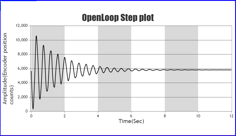
Fig. 4. Open loop step plot for 1 kg mass on Mass Spring Damper system without connecting the dashpot
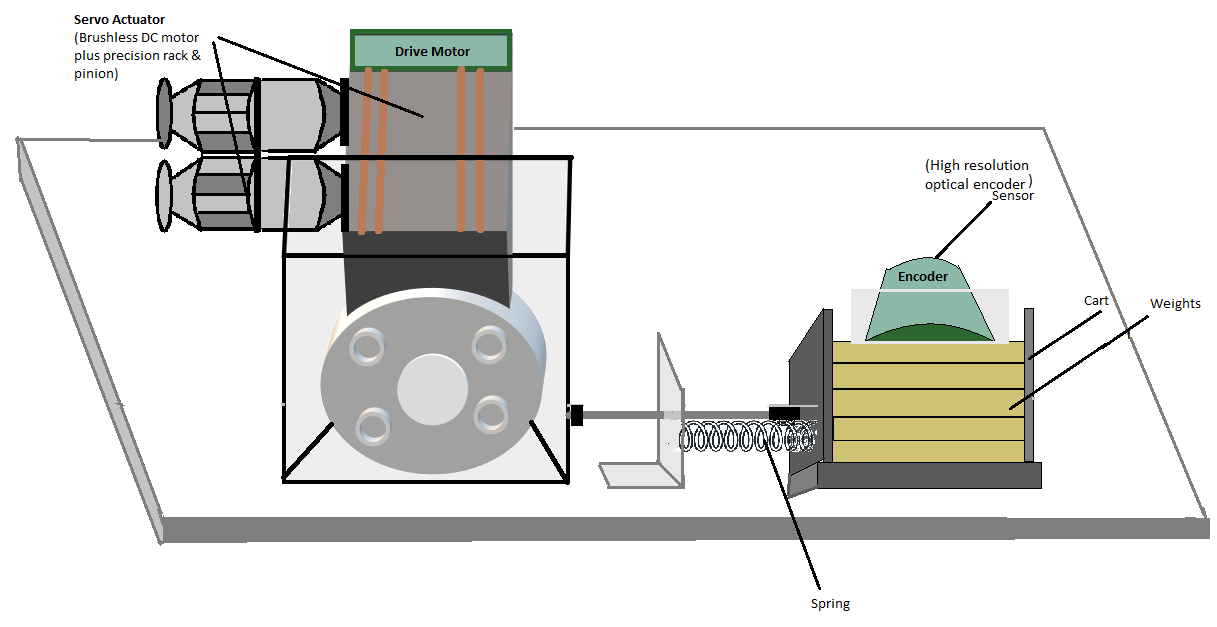
Fig. 5. Rectilinear Plant
The hardware gain, khw, of the system is comprised of the product
$$k_{hw} = k_c \ k_a \ k_t \ k_{mp} \ k_e \ k_{ep} \tag{7}$$
where the theoretical values are
kc, the DAC gain, = 10V / 32,768 DAC counts
ka, the Servo Amp gain, = approx 2 (amp/V)
kt, the Servo Motor Torque constant = approx 0.1 (N-m/amp)
kmp, the Motor Pinion pitch radius inverse = 26.25 m-1
ke, the Encoder gain, = 16,000 pulses / 2π radians
kep, the Encoder Pinion pitch radius inverse = 89 m-1
Controls section description:
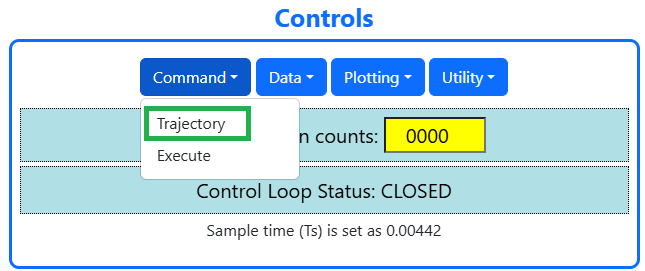
Fig. 6. Conrols Section in simulation page
This experiment needs support of PC controller which is shown in the 'Simulation' as 'Controls' section. This section contains some tabs named 'Command', 'Data', 'Plotting'
and 'Utility'.
- Command : The Command menu contains two pull-down options i.e. 'Trajectory' and 'Execute'.
- The Trajectory Configuration dialog box provides a selection of trajectory through which the apparatus can be maneuvered. Here it is 'Step'.
- After selecting the step trajectory followed by Setup, one enters a dialog box for the corresponding trajectory.
- Here 'Open loop step' needs to be selected.
- After clicking the 'Execute' option one dialog box is appeared. Here the user commands the system to execute the current specified trajectory.
- The user normally selects 'Run' here. The controller will begin execution of the specified trajectory.
- Once finished the data will be uploaded into the PC memory for plotting and saving.
- Data: The Data menu contains one pull-down option i.e. Setup Data Acquisition.
- An encoder is a sensor that converts a positional output into an electronic signal.
- In this experiment, encoder counts are used as the system units of position to follow the specified trajectory.
- In 'Setup Data Acquisition' dialog box user needs to select suitable option based on the instruction provided.
- The user must also select sampling period in multiples of the servo cycle. For example, the sample time Ts is 0.00442 seconds and 5 for your gather period here, then the selected data will be gathered once every fifth sample or once every 0.0221 seconds.
- Plotting: The 'Plotting' segment has two two pull-down options i.e. 'Setup Plot' and 'Plot Data'.
- Same like 'Setup Data Acquisition' dialog box user needs to select suitable option based on the instruction provided.
- The Setup Plot dialog box allows the acquired data to be plotted.
- The 'Plot Data' will provide response to the user or generates a plot of the selected item.
- Utility: The 'Utility' has one pull-down option i.e. 'Reset Controller' which enables the user to redo the experiment with different value of weights.