a. Least Mean Square (LMS) and Recursive Least Squares (RLS) Adaptive Filters

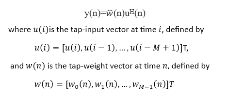
Least Mean Square (LMS) Adaptive Filter Concepts

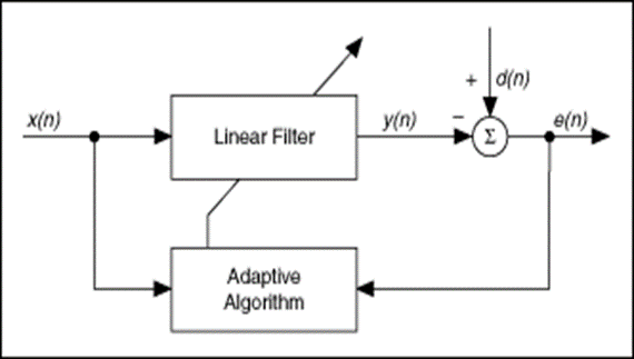
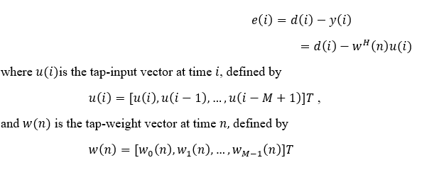
An adaptive filter is a computational device that iteratively models the relationship between the input and output signals of a filter. An adaptive filter self-adjusts the filter coefficients according to an adaptive algorithm.

Least Mean Squares (LMS) algorithms are a class of adaptive filters used to mimic a desired filter by finding the filter coefficients that produce the least mean square of the error signal (difference between the desired and the actual signal). It is a stochastic gradient descent method, meaning the filter adapts using only the error at the current time instant.

Signal Definitions

• x(n): Input signal to the linear filter
• y(n): Corresponding output signal
• d(n): Desired (reference) signal
• e(n): Error signal representing the difference between d(n) and y(n)

The linear filter may be a Finite Impulse Response (FIR) or Infinite Impulse Response (IIR) filter.
An adaptive algorithm iteratively adjusts the coefficients of the linear filter to minimize the power of the error signal e(n).

The LMS algorithm is one of several adaptive algorithms used to adjust FIR filter coefficients. Another important adaptive algorithm is the Recursive Least Squares (RLS) algorithm.

LMS Algorithm Steps

The LMS algorithm updates the coefficients of an adaptive FIR filter through the following steps:

1. Calculate the Filter Output

2. Calculate the Error Signal

e(n) = d(n) - y(n)

3. Update the Filter Coefficients

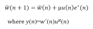
Where:

• μ: Step size of the adaptive filter
• w(n): Filter coefficient vector
• u(n): Filter input vector

Advantages of LMS

• Simple and easy to implement
• Low computational complexity
• Good convergence in stable environments
• Improved time-domain waveform tracking

Limitations of LMS

• Low convergence rate
• Poor performance at low signal-to-noise ratio (SNR)

Recursive Least Squares (RLS)

Adaptive filtering automatically adjusts filter coefficients to achieve desired filtering characteristics. The Recursive Least Squares (RLS) algorithm is a powerful adaptive filtering technique known for its rapid convergence and high accuracy.

RLS is widely used in applications such as:

• Noise cancellation
• Echo cancellation
• System identification

The goal of adaptive filtering is to minimize the difference between the desired signal and the actual output. The RLS algorithm achieves this by recursively minimizing a weighted least squares cost function using both past and present error samples.

Mathematical Foundation of RLS

The RLS algorithm minimizes the following cost function J(n):

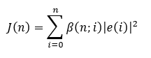
Where the error is defined as:

Here:

• e(i) is the difference between desired response d(i) and filter output y(i)
• The FIR filter tap weights remain fixed during the observation interval
• 1≤i≤n

The weighting factor β(n, i) satisfies:

0<β(n,i)≤1

Forgetting Factor

The weighting factor ensures older data is gradually “forgotten” to allow tracking of time-varying signals.

A commonly used weighting is the exponential forgetting factor:

β(n,i)=λ(n−i),i=1,2,…,n

Where:

• λ is close to but less than 1
• λ=1 → infinite memory (ordinary least squares)
• 1/1−λ → approximately represents the algorithm memory

RLS Initialization

The RLS algorithm is initialized as follows:

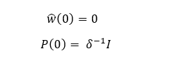
Where δ is the regularization parameter:

• Small δ → High SNR
• Large δ → Low SNR

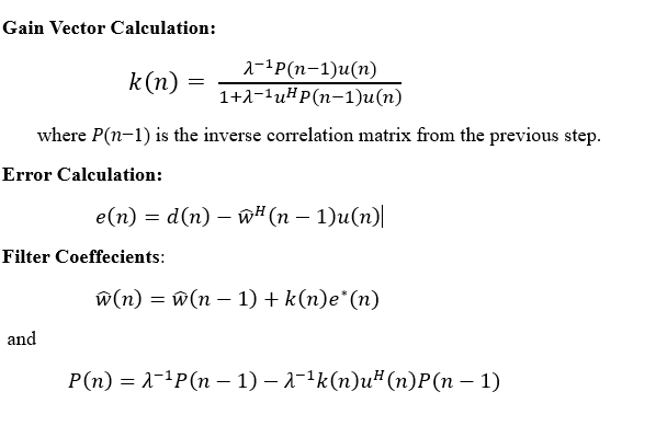
Recursive Update Equations

For each time instant n=1,2,… the following computations are performed:

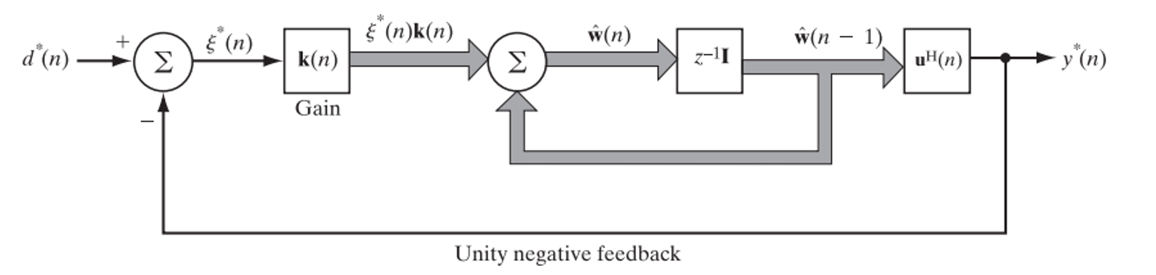
Signal Flow Graph

Advantages of RLS

• Very fast convergence
• High accuracy in coefficient estimation
• Excellent tracking of time-varying systems

Limitations of RLS

• High computational complexity
• Large memory requirement due to inverse correlation matrix storage

Comparison of LMS and RLS Adaptive Filters

Least Mean Squares (LMS) algorithms are the simplest adaptive filtering techniques and are easy to implement. Recursive Least Squares (RLS) algorithms offer superior performance and faster convergence at the cost of increased computational complexity.

RLS approaches the performance of the Kalman filter while requiring less throughput in signal processing.

Although LMS and RLS share the same signal paths and filter structure, they differ in how coefficients are adapted:

• LMS adapts based on instantaneous error
• RLS adapts using total accumulated weighted error

LMS uses a gradient-based approach with a step size μ:

• Small μ → Slow but stable convergence
• Large μ → Fast but potentially unstable

RLS minimizes a global least-squares cost function and adapts much faster.

Summary

• LMS is simple, stable, and computationally efficient but converges slowly
• RLS provides faster convergence and higher accuracy at increased computational cost
• LMS is suitable for low-resource systems
• RLS is preferred for high-performance and fast-tracking applications

b. Autoregressive Model

A statistical model is said to be autoregressive if it predicts future values based on past values. For example, an autoregressive model may be used to predict a stock’s future price based on its historical performance.

Basic Concept of Autoregressive Models

Autoregressive models operate under the premise that past values influence current values, which makes this statistical technique popular for analyzing natural phenomena, economics, and other time-varying processes.

Multiple regression models forecast a variable using a linear combination of predictors, whereas autoregressive models use a linear combination of past values of the same variable.

• AR(1) process: Current value depends on the immediately preceding value
• AR(2) process: Current value depends on the previous two values
• AR(0) process: Represents white noise, with no dependence between terms

There are various methods to estimate the coefficients of AR models, such as the least squares method.

Block Diagram of an Autoregressive Model

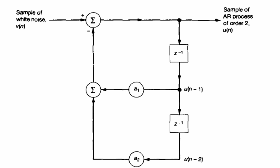
Second Order Autoregressive Process

Consider a second-order autoregressive (AR(2)) process that is real-valued.
The above figure illustrates the block diagram of the model used to generate this process.

The time-domain behavior of the AR(2) process is governed by the following second-order difference equation:

u(n) + a₁u(n-1) + a₂u(n-2) = v(n)

Where:

• u(n) is the output of the AR process
• a₁, a₂ are autoregressive coefficients
• v(n) is a white noise sequence with
  • Zero mean
  • Variance σ^2

Key Characteristics of AR Models

• Output depends on past outputs
• Suitable for time-series analysis
• Widely used in signal processing, economics, and forecasting
• Model order determines memory depth

Summary

• Autoregressive models predict current values using past observations
• AR(1), AR(2), and AR(0) represent increasing levels of dependency
• AR(2) models are governed by second-order difference equations
• White noise acts as the driving input to the system

c. Stochastic Processes

Stochastic Process Definition

• A stochastic process is a mathematical model that describes a sequence of random variables. The individual random variables in the sequence are usually called events.
• A stochastic or random process can be defined as a collection of random variables that is indexed by some mathematical set, meaning that each random variable of the stochastic process is uniquely associated with an element in the set.
• A stochastic process can be used to model the evolution of a physical system over time, or the evolution of a random variable over time.

---

Types of Stochastic Processes

There are four types of stochastic processes:

1. Discrete-time stochastic processes:
   These processes are characterized by a sequence of random variables, each of which takes on a finite set of values.

2. Continuous-time stochastic processes:
   These processes are characterized by a sequence of random variables, each of which takes on a continuous range of values.

3. Stationary stochastic processes:
   These processes are characterized by the fact that the statistical properties of the random variables do not change over time.

4. Non-stationary stochastic processes:
   These processes are characterized by the fact that the statistical properties of the random variables change over time.

---

Stationary Random Processes

A random process at a given time is a random variable, and in general, the characteristics of this random variable depend on the time at which the random process is sampled.

A random process X(t) is said to be stationary or strict-sense stationary if the probability density function (pdf) of any set of samples does not vary with time. In other words, the joint pdf or cumulative distribution function (cdf) of

X(t₁), … , X(tₖ)

is the same as the joint pdf or cdf of

X(t₁ + τ), … , X(tₖ + τ)

for any time shift τ and for all choices of t₁, … , tₖ.

In principle, it is difficult to determine if a process is stationary. Moreover, stationary processes cannot occur physically because real signals begin and end at finite times. Due to practical considerations, the observation interval is limited, and usually only first- and second-order statistics are used instead of joint pdfs and cdfs.

Since it is difficult to determine the complete distribution of a random process, analysis often focuses on partial yet useful descriptions such as the mean, autocorrelation, and autocovariance functions.

---

Wide-Sense Stationary (WSS) Processes

A random process X(t) is said to be wide-sense stationary (WSS) if:

1. The mean is constant:
   E[X(t)] = μ, independent of time

2. The autocorrelation function depends only on the time difference:
   τ = t₂ − t₁, and not on t₁ and t₂ individually

3. E[X²(t)] < ∞ (finite power condition)

That is,

Rₓ(t₁, t₂) = Rₓ(t₂ − t₁)

All strict-sense stationary processes are wide-sense stationary, but the converse is not always true. However, if a Gaussian random process is wide-sense stationary, then it is also stationary in the strict sense.

---

Non-Stationary Processes

In a covariance stationary stochastic process, the mean, variance, and autocovariance are assumed to be independent of time. In a non-stationary process, one or more of these assumptions does not hold.

A non-stationary process is characterized by a joint pdf or cdf that depends on the specific time instants t₁, … , tₖ. For a stationary random process, the mean and variance are constants and do not vary with time.

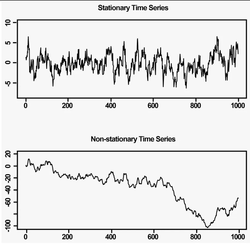
Data points are often non-stationary and may have means, variances, or covariances that change over time. Non-stationary behaviors can include trends, cycles, random walks, or combinations of these. Non-stationary data are generally unpredictable and difficult to model or forecast.

---