Pivot Selection in QuickSort

QuickSort is a Divide and Conquer algorithm that works by selecting a 'pivot' element and partitioning the array around it. The choice of pivot significantly affects the algorithm's performance.

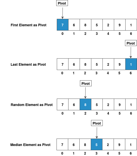
Common Pivot Selection Strategies

1. First Element as Pivot

   • Simple to implement
   • Poor performance on already sorted arrays

2. Last Element as Pivot

   • Most commonly used in implementations
   • Easy to understand and code

3. Random Element as Pivot

   • Provides good average-case performance
   • Helps avoid worst-case scenarios

4. Median as Pivot

   • Best theoretical choice
   • Requires additional computation to find median

Pictorial Representation of Pivot Selection

---

Array Partitioning Process

Goal: Given an array and a pivot element, rearrange the array so that:

• All elements ≤ pivot are on the left
• The pivot is in its correct sorted position
• All elements > pivot are on the right

Three-Part Division

After partitioning, the array is divided into three sections:

Partition 1	Partition 2	Partition 3
Elements ≤ pivot	Pivot element	Elements > pivot

---

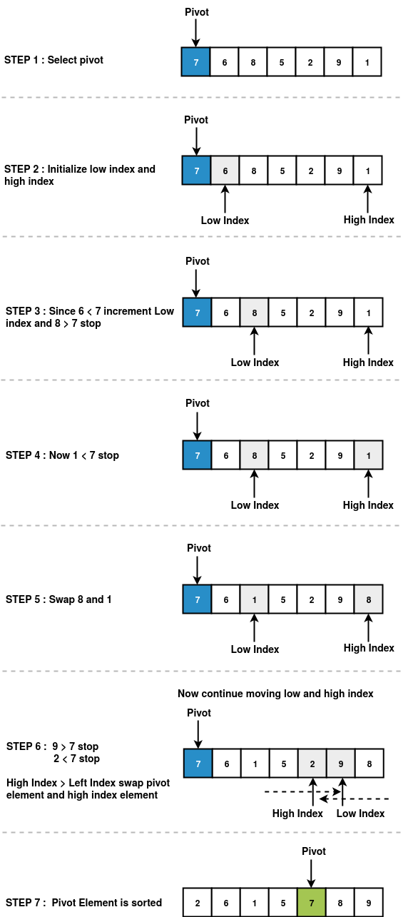
Partitioning Algorithm Steps

Step 1: Select Pivot

Choose a pivot using one of the strategies mentioned above.

Step 2: Initialize Pointers

• Low index (i): Points to the first element
• High index (j): Points to the last element (excluding pivot if it's the last element)

Step 3: Compare and Move Pointers

From the left (low index):

• If array[i] ≤ pivot, move i forward
• If array[i] > pivot, stop

From the right (high index):

• If array[j] > pivot, move j backward
• If array[j] ≤ pivot, stop

Step 4: Swap or Place Pivot

• If i < j: Swap array[i] and array[j], then repeat Step 3
• If i ≥ j: Partitioning is complete, place pivot at correct position

Step 5: Recursive Calls

Apply QuickSort recursively to both sub-arrays (left and right of the pivot).

---

Example Walkthrough

Initial Array: [64, 34, 25, 12, 22, 11, 90]
Pivot: 90 (last element)

1. Initialize: i = 0, j = 5 (pointing to 11)
2. Compare: Move pointers until elements need swapping
3. Partition: After processing: [64, 34, 25, 12, 22, 11, 90]
4. Result: All elements ≤ 90 are on the left, 90 is in correct position

Pictorial Representation of Partitioning Process

---

Key Points to Remember

✅ Partitioning is the core operation in QuickSort
✅ Pivot choice affects performance - random selection often works well
✅ In-place partitioning uses constant extra space
✅ After partitioning, pivot is in its final sorted position
✅ Recursively apply to sub-arrays on both sides of pivot

---

Time Complexity

• Best/Average Case: O(n log n) - when pivot divides array roughly equally
• Worst Case: O(n²) - when pivot is always the smallest/largest element
• Space Complexity: O(log n) - due to recursive call stack