Step 1: Understanding the Interface

When you open the simulation, you'll see three main sections:

• Left Panel (Control Panel): Contains all adjustable parameters and controls
• Center Area (Simulation Canvas): Displays the animated wavefunction
• Right Panel (Info Panel): Shows procedure steps, equations, and observations

---

Basic Experiment

Step 2: Set Initial Parameters

1. Set the Quantum Number (n) = 1 using the slider (this is the ground state)
2. Keep the Box Length (L) = 5 nm for initial observation
3. Set Wave Amplitude = 100 for clear visualization
4. Set Animation Speed = 5x for comfortable viewing

Step 3: Start the Simulation

1. Click the ▶ Start button to begin the simulation
2. Observe the wavefunction oscillating in time
3. Notice the status badge changes to "Running"
4. Use ⏸ Pause to freeze the animation at any point

Step 4: Observe the Ground State (n = 1)

• The wavefunction has 0 nodes (zero crossings inside the box)
• There is 1 antinode (peak) at the center
• Note the Energy value displayed in Live Measurements

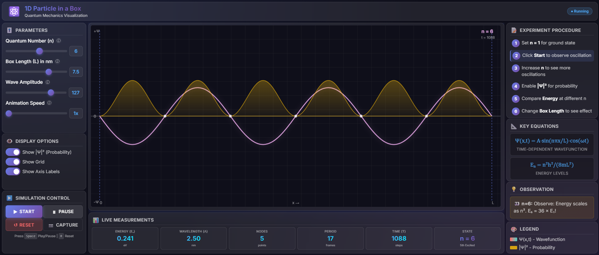
Fig. 1 Wave function and the Probability of the Particles trapped in 1D box.

---

Exploring Higher Energy States

Step 5: Increase Quantum Number

1. Gradually increase n from 1 to 10 using the slider
2. For each value of n, observe:
   • Number of peaks (antinodes) = n
   • Number of nodes = n - 1
   • Energy increases as n²

Step 6: Record Observations

Fill in the observation table for each quantum number:

n (Quantum Number)	Energy (eV)	Wavelength (nm)	No. of Nodes	No. of Peaks
1	0.015	10.00	0	1
2	0.060	5.00	1	2
3	0.135	3.33	2	3
4	0.241	2.50	3	4
5	0.376	2.00	4	5
6	0.542	1.67	5	6
7	0.737	1.43	6	7
8	0.963	1.25	7	8
9	1.218	1.11	8	9
10	1.504	1.00	9	10

---

Probability Density Analysis

Step 7: Enable Probability Display

1. In the Display Options section, toggle ON "Show |Ψ|² (Probability)"
2. Observe the yellow curve showing probability density as shown in fig.1
3. Compare with the wavefunction (gradient colored curve)

Step 8: Compare Wavefunction and Probability

• The probability density is always positive
• Probability is zero at nodes and maximum at antinodes
• The particle is most likely to be found at antinode positions

---

Box Length Investigation

Step 9: Vary Box Length

1. Keep n = 3 constant
2. Change Box Length (L) from 1 nm to 10 nm
3. Observe how:
   • Wavelength changes with box length
   • Energy decreases for larger boxes
   • The same number of nodes but spread differently

Step 10: Record Box Length Effect

Box Length L (nm)	Energy at n=3 (eV)	Wavelength (nm)
1	3.385	0.67
3	0.376	2.00
5	0.135	3.33
7	0.069	4.67
10	0.034	6.67

---

Additional Features

Step 11: Use Keyboard Shortcuts

• Press Spacebar to toggle Play/Pause
• Press R to Reset the simulation

Step 12: Capture Screenshots

1. Click the 📷 Capture button to save the current visualization
2. Use these for your lab report

Step 13: Reset and Repeat

1. Click the ↺ Reset button to return to initial state
2. Repeat the experiment with different parameter combinations

---

Analysis and Conclusion

Step 14: Plot Graph

Plot graphs of:

1. Energy (Eₙ) vs Quantum Number (n) - Should show quadratic relationship
2. Nodes vs Quantum Number (n) - Should show linear relationship (nodes = n-1)

Step 15: Write Inferences

Based on your observations, answer:

1. How does energy scale with quantum number?
2. What is the relationship between n and number of nodes?
3. How does box length affect the energy levels?
4. Where is the particle most likely to be found for each state?

---

Tips for Best Results

💡 Use the Pause button to closely examine wavefunction at specific times 💡 Compare different n values side by side using screenshots 💡 Toggle probability display to understand the physical meaning 💡 Experiment with different box lengths to see confinement effects