Periodic Signals
Fourier series of periodic signals
Fourier series theory says that many periodic signals can be represented in terms of sine and cosines and their harmonics in the given period. We can verify that any two signals in this set are orthogonal as discussed in the experiment Signal representation and orthogonality.
- Fourier Series Analysis: Given a periodic signal x(t) with time period T, analysis involves finding the Fourier series coefficients, x(t)→{ak,bk}
- Fourier Series Synthesis: Given Fourier series coefficients, synthesis involves reconstructing the periodic signal x(t)
Let x(t) be a periodic signal with time period (T=ω02π). Its Fourier Series coefficients are given as {ak,bk}, whereak=T2∫<T>x(t)cos(kω0t)dt k=1,2,...,∞bk=T2∫<T>x(t)sin(kω0t)dt k=1,2,...,∞a0=T1∫<T>x(t)dt (average value of signal in one period)The set of signals {1, cos(kω0t), sin(kω0t)}k=0,1,..,∞ forms a basis for the space of all periodic signals with time-period T=F01=ω02π,x(t)=a0+k=1∑∞akcos(kω0t)+k=1∑∞bksin(2πkω0t)For real-valued signals x(t), the coefficients {ak,bk} are real valued.
Partial reconstruction
The signal x(t) can be partially reconstructed using the first R Fourier series coefficients {ak,bk},k=0,1,.. R as follows, x^(t)=a0+k=1∑Rakcos(2πkf0t)+k=1∑Rbksin(2πkf0t)The signal reconstruction error is given as e(t)=x(t)−x^(t).
Quasi-periodic signals
Many naturally occurring signals are close to periodic, called quasi-periodic. For example, the human heart beat. Quasi periodic signals appear to be periodic but have small fluctuations in the period over time. An example of a noisy human heart signal (also called electrocardiogram, i.e., ECG) is shown below.
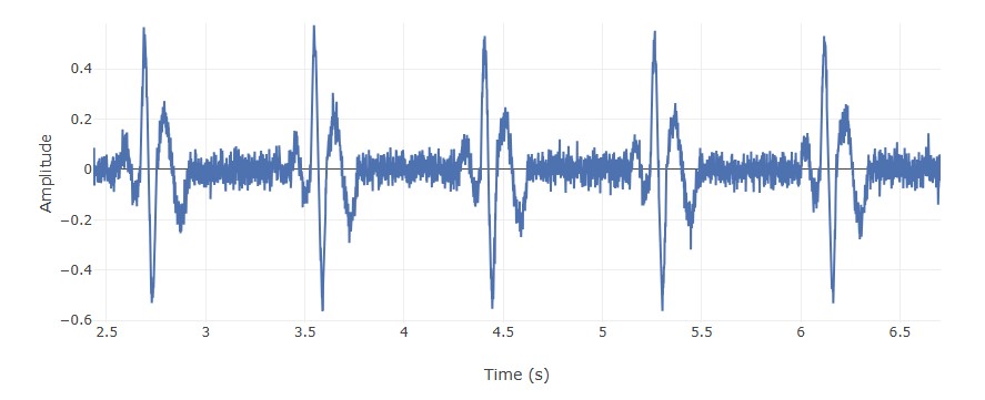
How does one go about finding the (approximate) time-period of such signals?
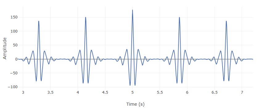
For the ECG signal above, a simple method could be measure the time intervals between the consecutive sharp peaks and average them. Such a method works well if the given signal has a repeating distinguishing feature (for example sharp peaks). In absence of such features, finding the time-period can be difficult from the signal. A simple trick to obtain distinguishing features is to correlate the given signal with itself. The correlation signal will have peaks when the various periods overlap. The correlation signal for the above ECG signal is shown below.
Why sinusoids?
Having learned about Fourier series, one can ask the follow up question - are sinusoids the only orthogonal basis that can be used to represent periodic signals? The answer is no. In fact, the above equations correspond to what is known as trigonometric Fourier series. They can be generalized to complex Fourier series which use periodic complex sinusoids as basis.
Given a set of harmonically related periodic basis signals, many general periodic signals can be represented using these basis signals. For example, consider a square wave of period T. Along with all its harmonics, this forms an orthogonal basis which can represent many periodic signals. The analysis and synthesis equations to obtain a series decomposition using these signals will be different from those of Fourier series.
Fourier series example
Compute the Fourier series coefficients of the square wave below:
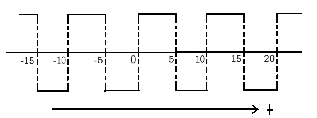
x(t)={30<t<5−35<t<10
Solution:
a0=T1∫0Tx(t)dt= 0
ak=T2∫2−T2Tx(t)cos(kω0t)dt
=102∫−55x(t)cos(kω0t)dt
=51[∫−50x(t)cos(kω0t)dt+∫05x(t)cos(kω0t)dt]
=51[−3∫−50cos(kω0t)dt+3∫05cos(kω0t)dt]
=0
Thus we have, ak=0 ∀ k=1,2...∞. Since x(t) is an odd signal, we get ak=0, which shows that there are no cosine terms in the Fourier representation of x(t).
bk=T2∫2−T2Tx(t)sin(kω0t)dt where ω0=102π
=102∫−55x(t)sin(kω0t)dt
=51[∫−50x(t)sin(kω0t)dt+∫05x(t)sin(kω0t)dt]
=51[−3∫−50sin(kω0t)dt+3∫05sin(kω0t)dt]
=kπ3[1−2cos(kπ)+cos(2kπ)]
=kπ6[1−cos(kπ)]
=kπ6[1−(−1)k]
bk={kπ120if k is oddif k is even
Now, x(t) can be represented as x(t)=∑k=2r−1r=1,..∞kπ12sin(kω0t).
