
Perceptron
Theory
Introduction to Perceptron
The perceptron is the simplest form of artificial neural network, invented by Frank Rosenblatt in 1958. It is a binary classifier that learns to separate data points into two classes using a linear decision boundary. A perceptron computes a weighted sum of its inputs, adds a bias term, and applies a step activation function to produce a binary output. The basic structure and working of a single-layer perceptron are illustrated in Fig. 1.
"A perceptron is a linear classifier that makes predictions using a weighted combination of input features followed by an activation function."
A single-layer perceptron consists of:
1. Inputs (x₁, x₂, ..., xₙ)
The features or data values that the perceptron receives to make decisions. These are like the raw information fed into the model. These input nodes and their connections to the perceptron are shown in Fig. 1.
Example: For the XOR problem, we have two binary inputs x₁ and x₂, each of which can be either 0 or 1.
2. Weights (w₁, w₂, ..., wₙ)
These are Importance scores that determine how much each input contributes to the final prediction. A larger weight (positive or negative) means that the input has a greater influence. The weighted connections between the inputs and the summation unit are shown in Fig. 1.
- Each input gets its own weight, acting as a multiplier for that feature
- Weights control the angle or tilt of the decision boundary line
3. Bias (b)
An adjustable constant added to the weighted sum that shifts the position of the decision boundary.
- Bias shifts the position of the decision boundary without changing its orientation, allowing the perceptron to better separate the classes.
- Bias controls the position or shift of the decision boundary line
Key Difference Between Weights and Bias:
- Weights determine the slope, how steep the line is and its direction
- Bias determines the position, where the line sits in the coordinate space
Together they define a complete line, similar to , where weights act like the slope and bias acts like the y-intercept . The bias term (representing the weight of the bias connection) is denoted as as seen in Fig. 1.
4. Net Input (Weighted Sum)
The perceptron combines all inputs, weights, and bias into a single numerical value:
This can be thought of as calculating a "score" — multiply each input by its weight, sum them all together, then add the bias. This score determines the predicted class. The summation operation () is shown in Fig. 1.
5. Activation Function (Step Function)
The activation function converts the numerical score into a binary decision:
- If the score is positive or zero → predict Class 1
- If the score is negative → predict Class 0
- This creates a threshold at z = 0 where the perceptron switches between classes
- The resulting decision boundary is always a straight line (linear), which is why perceptron can only solve linearly separable problems
The step activation function and output of the perceptron are shown in Fig. 1.
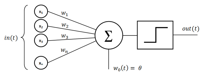
Fig. 1: Architecture of a Single-Layer Perceptron showing inputs, weights, summation unit, and step activation function.
Perceptron Learning Algorithm
The perceptron learns through a simple trial-and-error process. It makes predictions, checks if they are correct, and adjusts its parameters when it makes mistakes. This is called supervised learning because we provide the correct answers during training.
The Learning Process:
Step 1: Make a Prediction
The perceptron calculates its weighted sum and makes a prediction:
Step 2: Check if the Prediction is Correct
Compare the predicted output () with the actual correct label ():
- If : The prediction was correct, no changes needed
- If : The perceptron predicted 0 but should have predicted 1 (underestimated)
- If : The perceptron predicted 1 but should have predicted 0 (overestimated)
Step 3: Update the Weights (Learn from Mistakes)
When the perceptron makes an error, it adjusts each weight to reduce that error:
where:
- (Learning Rate): Controls how big the adjustment steps are
- : Tells us the direction and magnitude to adjust
- : The input value that contributed to this weight
Example: If the perceptron predicted 0 but the answer was 1, the error is +1, so weights connected to active inputs (xᵢ = 1) increase, making the perceptron more likely to predict 1 next time.
Step 4: Update the Bias (Shift the Boundary)
The bias is adjusted similarly, but without multiplying by any input:
This shifts the decision boundary to better separate the classes.
Step 5: Repeat for All Training Examples
The perceptron goes through every data point in the training set, making predictions and adjusting weights. One complete pass through all data points is called an epoch.
Step 6: Train for Multiple Epochs
The process repeats for several epochs. With each epoch:
- The decision boundary moves and rotates
- Classification accuracy typically improves
- The perceptron gets closer to the correct solution (if one exists)
Step 7: Convergence or Stopping
Training stops when either:
- Convergence: All training examples are classified correctly (only possible for linearly separable data)
- Maximum epochs reached: We have trained for a fixed number of epochs
Important Note: For linearly separable problems like AND or OR gates, the perceptron will eventually find a perfect solution. However, for non-linearly separable problems like XOR, the perceptron will never converge and will continue making errors indefinitely, which is exactly what we observe in this experiment.
Linear Separability
A dataset is linearly separable if there exists a straight line (in 2D), plane (in 3D), or hyperplane (in higher dimensions) that can perfectly separate the two classes. A single-layer perceptron can only learn linearly separable patterns.
Examples of linearly separable problems:
- AND gate: (0,0) → 0, (0,1) → 0, (1,0) → 0, (1,1) → 1
- OR gate: (0,0) → 0, (0,1) → 1, (1,0) → 1, (1,1) → 1
Examples of non-linearly separable problems:
- XOR gate: (0,0) → 0, (0,1) → 1, (1,0) → 1, (1,1) → 0
The XOR Problem
XOR (Exclusive OR) is a Boolean logic function that outputs 1 when the inputs are different and 0 when they are the same. The XOR truth table is:
| x₁ | x₂ | XOR Output |
|---|---|---|
| 0 | 0 | 0 |
| 0 | 1 | 1 |
| 1 | 0 | 1 |
| 1 | 1 | 0 |
When plotted in 2D space, the XOR problem shows a diagonal pattern where:
- Points (0,0) and (1,1) belong to Class 0 (blue)
- Points (0,1) and (1,0) belong to Class 1 (red)
No matter how we adjust w₁, w₂, and b, we cannot draw a single straight line that achieves this separation. The perceptron will keep updating its weights indefinitely, oscillating between different incorrect solutions, never achieving 100% accuracy.
The solution came with the development of Multi-Layer Perceptrons (MLPs) with hidden layers and non-linear activation functions. A two-layer neural network, consisting of one hidden layer containing at least two neurons and one output layer, can solve the XOR problem. The hidden layer creates multiple linear decision boundaries, and their combination enables the network to learn non-linearly separable patterns correctly.
Merits of Perceptron
Simplicity: Easy to understand and implement.
Computational Efficiency: Fast training and prediction for linearly separable problems.
Foundation: Forms the basis for understanding more complex neural networks.
Interpretability: The decision boundary can be easily visualised and understood.
Demerits of Perceptron
Linear Limitation: Cannot solve non-linearly separable problems like XOR.
Binary Classification Only: Limited to two-class problems in basic form.
Sensitive to Feature Scaling: Performance can be affected by input feature scales.
No Convergence for Non-separable Data: May oscillate indefinitely without reaching a solution.