
Multiplexing vs. Diversity
In the previous two experiments, we have learned about spatial diversity and multiplexing techniques separately. It is understood that the diversity improves the received SNR which helps to reduce the bit error rate (BER), whereas the spatial multiplexing enables the transmission of parallel data streams so that the transmission capacity can be improved.
While spatial diversity and spatial multiplexing serve different performance objectives, they both utilize the same spatial Degrees of Freedom (DoF) offered by the MIMO channel. Diversity techniques exploit the spatial dimension to improve reliability, whereas multiplexing techniques exploit it to increase transmission rate. Since the total available DoF is limited by the rank of the channel matrix, a fundamental trade-off arises between reliability and data rate.
In multiplexing, we decompose the MIMO channel into parallel SISO channels. The SNRs associated with these parallel streams depend on the eigenvalues of channel covariance matrix. Thus, there is a possibility that the SNR of a particular stream is poor which may result in its poor BER performance. To overcome this, the spatial degree of freedom offered by the channel can be partially used for diversity gain with some reduction in the multiplexing gain. This will improve SNR performance at the cost of the reduced number of parallel streams, which essentially leads to "diversity vs. multiplexing trade-off". The choice of diversity and multiplexing orders will depend on the application. For instance, a higher multiplexing order will provide a high transmission rate but with poor BER performance. Whereas, setting a high diversity order will improve BER performance but at the cost of reduced data rate. Therefore, such diversity vs. multiplexing trade-off can be also viewed as the trade-off between transmission rate and BER.
Comparison Between Spatial Multiplexing and Spatial Diversity
The fundamental differences between spatial multiplexing and spatial diversity are summarized in the following table for better understanding:
| Feature | Spatial Multiplexing | Spatial Diversity |
|---|---|---|
| Primary Objective | Increase data rate | Improve reliability (reduce BER) |
| Use of DoF | Used for parallel streams | Used for creating diverse paths |
| Capacity | High capacity | Moderate capacity |
| BER Performance | Higher BER (at same SNR) | Lower BER |
| SNR | Low/moderate, same as SISO | Improved by comibining |
| Suitable For | High data rate applications | Reliable communication systems |
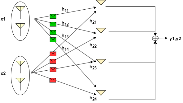
Consider the scenario illustrtated in the following figure, where the transmitter has 4 transmit antennas and the reciever has 4 receive antennas. If the multiplexing gain of 2 is desired, then antennas can be divided into 2 groups so that each group stream can utilize 2 antennas for the diversity as shown in the figure.
For a given multiplexing gain , then the optimal diversity gain that can be achieved is given as
The above expression clearly shows that as the multiplexing gain increases, the diversity gain decreases. This inverse relationship mathematically characterizes the diversity–multiplexing trade-off (DMT). At one extreme, when , maximum diversity is achieved. At the other extreme, when , the diversity gain becomes zero.
The optimal multiplexing and diversity trade-off can be visualized from the following plot [2].
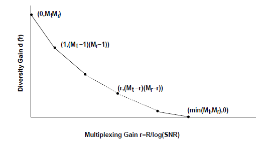
The curve illustrates that one cannot simultaneously maximize both diversity and multiplexing gains. Instead, practical systems must select an operating point depending on application requirements such as target data rate, acceptable BER, and channel conditions.