
To understand and implement a Multi-Layer Perceptron (MLP) with focus on architecture, activation functions, and training
Introduction
The Multi-Layer Perceptron, commonly referred to as MLP, consists of fully connected dense layers designed to transform input dimensions into the desired output dimensions. Essentially, it represents a neural network with multiple layers. In the construction of a neural network, neurons are interconnected, forming a complex web where the outputs of certain neurons serve as inputs for others. This interconnected structure allows for intricate information processing, making the Multi-Layer Perceptron a versatile and powerful tool in the realm of neural networks.
MLP consists of an input layer, where each input corresponds to a single neuron or node. The MLP also includes an output layer, with a dedicated node for each output. In addition to the input and output layers, the MLP can incorporate multiple hidden layers, each comprising a flexible number of nodes. The versatility of an MLP lies in its ability to have any number of hidden layers, and within each hidden layer, any desired number of nodes can be configured.
Why MLP?
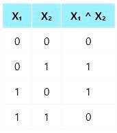
The XOR (exclusive OR) problem is a classic example that highlights the limitations of a Single-Layer Perceptron (SLP), in solving non-linearly separable problems. The XOR problem involves two binary inputs (0 and 1) and produces a binary output based on the exclusive OR logic:
The goal is to find a decision boundary that separates the two classes (output 0 and output 1).
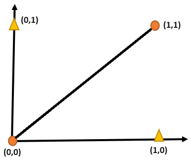
From the above illustration, it's evident that the gold triangle above the linearly separable line overlaps with the orange dot, making it clear that achieving linear separability of data points is unattainable using XOR logic alone. To address this limitation, the Multi-Layer Perceptron (MLP) comes into play. The incorporation of multiple layers and non-linear activation functions in neural networks makes it suitable for tackling complex tasks.
Basic Architecture
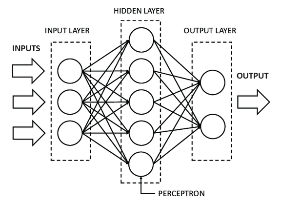
- A Multi-layer perceptron consists of an input layer, a hidden layer, and an output layer.
- The input layer is responsible for receiving the initial data, with each input corresponding to a neuron or node. These nodes act as receptors for the various features or attributes of the input data.
- The hidden layer consists of multiple neurons, and the connections between neurons are characterized by weights that adjust during the training process. These weights determine the strength and direction of the signal as it passes through the network.
- The output layer layer synthesizes the information processed in the hidden layers to produce the final result or prediction. In classification tasks, each node in the output layer often represents a different class or category, and the neuron with the highest activation is considered the predicted class.
The schematic diagram below illustrates the architecture of a Multi-Layer Perceptron, showcasing its input, hidden, and output layers along with the connections between nodes.
Forward Propagation
It is the process where the input data is fed through the network in a forward direction, layer-by-layer, until it generates the output.
Activation function
Activation functions introduce non-linearity to the network. Common choices include the sigmoid, hyperbolic tangent (tanh), and Rectified Linear Unit (ReLU). The non-linear activation allows the network to learn and model complex relationships in the data.
The activation of the neuron is computed in two steps:
- We first compute the net input of the neuron as the weighted sum of its incoming inputs. The formula is expressed as the sum of the products of each input value (X) and its corresponding weight (W), which is represented as:
∑(X * W) - We now apply the activation function to the net input to get the neuron’s activation. The activation function introduces non-linearity to the neuron's response, allowing it to capture complex patterns in the data. The choice of activation function depends on the problem and desired behavior of the model.
-
Sigmoid Function: It is a function which is plotted as ‘S’ shaped graph.
-
Equation:
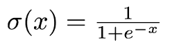
Fig. 3 Sigmoid equation - Nature: Non-linear
- Value Range: 0 to 1
- Uses: Usually used in output layer of a binary classification, where result is either 0 or 1, as value for sigmoid function lies between 0 and 1 only so, result can be predicted easily to be 1 if value is greater than 0.5 and 0 otherwise.
-
Equation:
-
Tanh Function: The activation that works almost always better than sigmoid function is Tanh function also known as Tangent Hyperbolic function. It’s actually mathematically shifted version of the sigmoid function.
-
Equation:
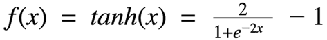
Fig. 4 Tanh equation - Nature: Non-linear
- Value Range: -1 to 1
- Uses: Usually used in hidden layers of a neural network as it’s values lies between -1 to 1 hence the mean for the hidden layer comes out be 0 or very close to it, hence helps in centering the data by bringing mean close to 0. This makes learning for the next layer much easier.
-
Equation:
-
ReLU Function: It Stands for Rectified linear unit. Chiefly implemented in hidden layers of Neural network.
-
Equation:
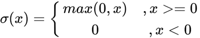
Fig. 5 ReLU equation - Nature: Non-linear
- Value Range: [0, inf)
- Uses: ReLu is less computationally expensive than tanh and sigmoid because it involves simpler mathematical operations.
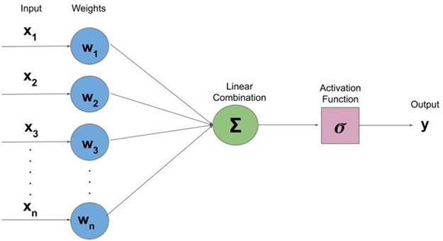
Fig. 6 Pictorial representation of computing activation of the perceptron -
Equation:
-
Sigmoid Function: It is a function which is plotted as ‘S’ shaped graph.
XOR Function using Artificial Neural Network (ANN)
The XOR (Exclusive OR) function is a fundamental logic function that outputs 1 only when the inputs are different. However, it is important to note that XOR is not linearly separable — meaning it cannot be represented using a single-layer perceptron.
To learn XOR, we use a multi-layer perceptron (MLP) — a neural network with one hidden layer.
Rewriting XOR Function
We can rewrite XOR as a combination of two linearly separable functions:
Now let’s interpret this expression step by step:
- Neuron 1 can learn the function A . B′
- Neuron 2 can learn the function A′ . B
- The output neuron performs an OR operation on these two results.
XOR Truth Table
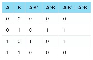
As we can see from the table, XOR gives an output of 1 only when one input is 1 and the other is 0. Hence, it requires combining two different linear functions using a hidden layer — making it a classic example of a non-linearly separable problem.
Backpropagation
It is the process of updating the weights and biases in the network based on the calculated gradients of the loss function with respect to these parameters. It involves moving backward through the network, adjusting the weights to reduce the error.
Some common applications of MLPs
- Image Recognition: MLPs are used for image classification tasks, such as identifying objects in images.
- Natural Language Processing: MLPs are employed in tasks such as sentiment analysis, text classification, and language translation. They can learn and extract features from textual data, making them valuable in NLP applications.
- Medical Diagnosis: MLPs are used in medical image analysis for tasks like tumor detection and classification. They can learn to recognize patterns in medical images, aiding in diagnosis.
- Speech Recognition: MLPs are utilized in speech recognition systems to convert spoken language into text. They can process and recognize patterns in audio data, enabling accurate transcription.
Advantages
- Non-Linearity: MLPs can model complex non-linear relationships within data, making them effective for tasks that involve intricate patterns.
- Scalability: MLPs can scale to handle large datasets and complex problems by adjusting the number of layers and neurons.
- Versatility: MLPs are versatile and can be applied to a wide range of tasks, including classification, regression, and pattern recognition.
- Generalization: With proper training and regularization, MLPs can generalize well to new, unseen data, demonstrating their ability to capture underlying patterns.
Disadvantages
- Computational Intensity: Training large and deep MLPs can be computationally intensive and may require significant resources, especially for complex tasks.
- Initialization Challenges: Choosing appropriate initial weights can be challenging, and poor initialization may lead to slow convergence or training failure.
- Need for Large Datasets: MLPs, especially deep architectures, may require large amounts of labeled data to effectively learn complex patterns and prevent overfitting.
- Hyperparameter Sensitivity: MLPs often have several hyperparameters, and their performance can be sensitive to choices such as learning rates, number of layers, and number of neurons, requiring careful tuning.