Theory

Introduction to Feedforward Neural Networks

A Multilayer Perceptron (MLP) is a class of deep learning model within feedforward neural networks, designed to learn a mapping between input data and corresponding output targets, expressed as

$$\hat{y} = f(x; \theta),$$

where $x$ represents the input features, $\hat{y}$ denotes the predicted output, and $\theta$ comprises the model parameters, including weights and biases. In classification tasks, the model assigns inputs to discrete classes, while in regression it predicts continuous values. A feedforward network is characterised by the unidirectional flow of information from the input layer through one or more hidden layers to the output layer, without any feedback connections, making it suitable for standard prediction tasks. The objective of such networks is to approximate an underlying target function $f^*$. For instance, in a classification task, the network learns a mapping

$$y = f^*(x),$$

in classification problems. A layered feedforward network ensures that all paths from input to output pass through the same number of layers, and it is considered fully connected when each neuron in one layer is linked to every neuron in the next. The key strength of MLPs lies in their ability to model complex, non-linear relationships and to generalise effectively to unseen data when trained on representative datasets.

Architecture of MLP

An MLP consists of multiple layers arranged sequentially:

• Input layer: accepts raw input features.
• Hidden layers: perform intermediate transformations.
• Output layer: produces the final prediction.

Each neuron in a layer is connected to every neuron in the next layer, forming a fully connected network. A network is called a layered feedforward network if every path from input to output passes through the same number of layers. Hidden layers are responsible for learning useful intermediate representations from the data.

Up to now, neural networks have been described as models in which the output of one layer is used as the input to the next layer; such architectures are called feedforward neural networks. In a pure feedforward network, information is always fed forward, never fed back, so there are no recurrent feedback loops. This can also be shown in Figure 1.

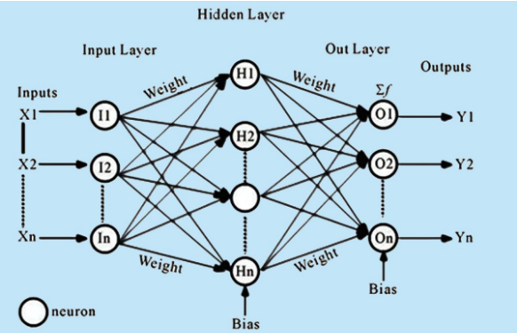
Figure 1 – Feed-Forward Neural Network Architecture (Source: Based on the standard multilayer perceptron model as presented in Goodfellow, Bengio & Courville, Deep Learning, MIT Press, 2016)

Mathematical Representation of MLP

Let the network consist of $L$ layers. The computation at each layer is performed in two steps.

Step 1: Linear Transformation

$$z^{(l)} = W^{(l)} h^{(l-1)} + b^{(l)}$$

Step 2: Non-linear Activation

$$h^{(l)} = \rho(z^{(l)})$$

where:

• $W^{(l)}$ is the weight matrix of layer $l$,
• $b^{(l)}$ is the bias vector,
• $\rho(\cdot)$ is the activation function such as ReLU, sigmoid, or tanh,
• $h^{(l)}$ is the output of layer $l$,
• $h^{(0)} = x$, the input vector.

The overall network is a composition of such transformations:

$$\Phi(x) = W_L \rho \!\left( W_{L-1} \rho \!\left( \cdots \rho(W_1 x + b_1) \cdots \right) + b_{L-1} \right) + b_L$$

This formulation shows that an MLP is built by stacking linear and non-linear transformations layer by layer.

Forward Propagation

Forward propagation is the process of passing input data through the network layer by layer. The input $x$ is transformed using weights, biases, and activation functions until the final output $\hat{y}$ is produced. In a feedforward neural network, information flows forward from the input to the output, and this process defines how predictions are generated.

For a typical MLP, the layer-wise computation can be written as:

$$h_1 = \rho(W_1 x + b_1)$$

$$h_2 = \rho(W_2 h_1 + b_2)$$

$$\hat{y} = g(W_L h_{L-1} + b_L)$$

where $g(\cdot)$ denotes the output activation function. In a classification task, $g(\cdot)$ is usually softmax. The forward pass is also the stage at which the prediction is produced before the loss is computed.

Loss Function (Error Measurement)

To evaluate how well the model performs, a loss function is used. It measures the difference between the predicted output $\hat{y}$ and the actual output $y$. The goal of training is to minimise this loss function so that predictions become closer to the true targets.

For regression problems, the least-squares loss is commonly used:

$$J(\theta) = \frac{1}{2} \| y - \hat{y} \|^2$$

For classification problems, cross-entropy loss is used. Since the Iris dataset in this experiment is a multi-class classification problem, categorical cross-entropy is appropriate:

$$J(\theta) = -\sum_{i=1}^{C} y_i \log(\hat{y}_i)$$

where:

• $y_i$ is the true one-hot encoded label,
• $\hat{y}_i$ is the predicted probability for class $i$,
• $C$ is the number of classes,
• $\theta$ represents all model parameters.

This loss function quantifies how far the predicted probability distribution is from the true class distribution.

Backpropagation (Learning Mechanism)

Backpropagation is the core algorithm used to train an MLP. It computes how the loss changes with respect to each parameter in the network. More precisely, the objective is to compute gradients of the cost function $J(\theta)$ with respect to the weights and biases. This is done using the chain rule of differentiation.

The gradients computed during backpropagation include:

$$\frac{\partial J(\theta)}{\partial W^{(l)}}, \quad \frac{\partial J(\theta)}{\partial b^{(l)}}$$

The process can be described as follows:

1. Compute the error at the output layer.
2. Propagate the error backward through the hidden layers.
3. Compute the gradient of the loss with respect to each parameter.

These gradients are then used to update the model parameters during training.

Parameter Update (Optimisation)

Once gradients are computed, the parameters are updated using gradient descent:

$$\theta \leftarrow \theta - \eta \frac{\partial J(\theta)}{\partial \theta}$$

where $\eta$ is the learning rate. This update rule moves the parameters in the direction that reduces the loss function.

Common optimisers include:

• Stochastic Gradient Descent (SGD)
• RMSprop
• Adam

These optimisation methods differ in how they scale or adapt the updates, but they all aim to minimise the same cost function $J(\theta)$.

Optimisation Algorithms

Common optimisation algorithms used for training neural networks include Stochastic Gradient Descent (SGD), RMSprop, and Adam. These methods aim to minimise the cost function $J(\theta)$ by iteratively updating the model parameters $\theta$. Although all three algorithms optimise the same objective function, they differ in how they compute and scale parameter updates, which affects convergence speed and stability.

Stochastic Gradient Descent (SGD)

Stochastic Gradient Descent (SGD) is one of the simplest and most widely used optimisation techniques. It updates the model parameters using the gradient of the loss function computed over a mini-batch of training samples. The update rule is given by

$$\theta_{t+1} = \theta_t - \eta \nabla_\theta J(\theta_t),$$

where $\eta$ is the learning rate and $\nabla_\theta J(\theta_t)$ represents the gradient of the cost function with respect to the parameters at iteration $t$. Although SGD is computationally efficient, it may converge slowly and can exhibit oscillations, particularly in regions where the loss surface is highly curved.

RMSprop

RMSprop is an adaptive learning rate method that improves upon SGD by scaling the parameter updates based on the magnitude of recent gradients. It maintains an exponentially weighted moving average of the squared gradients, defined as

$$v_t = \beta v_{t-1} + (1 - \beta)(\nabla_\theta J(\theta_t))^2,$$

where $\beta$ is the decay rate. The parameter update rule is then given by

$$\theta_{t+1} = \theta_t - \frac{\eta}{\sqrt{v_t} + \epsilon} \nabla_\theta J(\theta_t),$$

where $\epsilon$ is a small constant added to ensure numerical stability. By normalising the gradient, RMSprop helps stabilise the learning process and is particularly effective when dealing with non-stationary objectives.

Adam (Adaptive Moment Estimation)

Adam is an advanced optimisation algorithm that combines the benefits of momentum and adaptive learning rates. It computes both the first moment and the second moment of the gradients. The moment estimates are given by

$$m_t = \beta_1 m_{t-1} + (1 - \beta_1) \nabla_\theta J(\theta_t),$$

$$v_t = \beta_2 v_{t-1} + (1 - \beta_2)(\nabla_\theta J(\theta_t))^2,$$

where $\beta_1$ and $\beta_2$ are decay rates. These estimates are bias-corrected as follows:

$$\hat{m}_t = \frac{m_t}{1 - \beta_1^t}, \quad \hat{v}_t = \frac{v_t}{1 - \beta_2^t}.$$

The parameter update rule is then given by

$$\theta_{t+1} = \theta_t - \frac{\eta}{\sqrt{\hat{v}_t} + \epsilon} \hat{m}_t.$$

Adam is widely used due to its efficiency, robustness, and ability to converge quickly in practice.

Training Workflow

The entire training process consists of repeating the following steps:

1. Forward propagation to compute predictions.
2. Loss computation to measure prediction error.
3. Backpropagation to compute gradients.
4. Parameter update using an optimisation algorithm.

This cycle is repeated for multiple epochs until the model converges or reaches a predefined stopping condition.

These models are called feedforward because information flows through the function being evaluated from $x$, through the intermediate computations used to define $f$, and finally to the output $\hat{y}$. There are no feedback connections in which the outputs of the model are fed back into itself.

I. Gradient-Based Learning: For feedforward neural networks, it is important to initialise all weights to small random values; biases may be initialised to zero or to small positive values. Iterative gradient-based optimisation algorithms, such as SGD, RMSprop, and Adam, are used to train feedforward networks and deep models.

II. Learning XOR: To illustrate the capabilities of feedforward networks, consider the XOR function. XOR returns 1 when exactly one of $x_1$ or $x_2$ is 1, and 0 otherwise. Learning XOR demonstrates that an MLP with a hidden layer can represent non-linearly separable functions. To make the idea of a feedforward network more concrete, we begin with an example of a fully functioning feedforward network on a very simple task: learning the XOR function. The XOR function ("exclusive or") is an operation on two binary values, $x_1$ and $x_2$. When exactly one of these binary values is equal to 1, the XOR function returns 1. Otherwise, it returns 0. The XOR function provides the target function $y = f^*(x)$ that we want to learn. Our model provides a function $y = f(x; \theta)$, and our learning algorithm adapts the parameters $\theta$ to make $f$ as similar as possible to $f^*$.

The process of forward propagation from input to output and backward propagation of errors is repeated several times until the error gets below a predefined threshold. The whole process is represented in the following diagram:

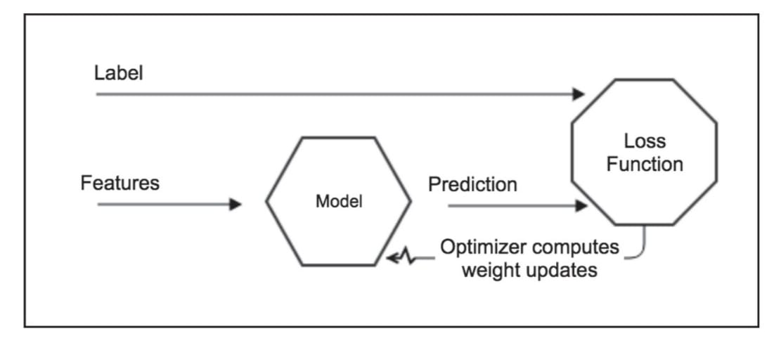
Figure 2- MLP Process both Forward and Backpropagation (Source: Antonio Gulli, Sujit Pal, Deep Learning with Keras)

The forward and backward propagation process is repeated until the error falls below a predefined threshold. The model is updated to progressively minimise the loss function. In a neural network, individual neuron outputs matter less than the collective behaviour of the weights in each layer, as shown in Figure 2; the network adjusts its internal weights so that prediction accuracy increases. Using appropriate features and high-quality labels is fundamental for reducing bias and improving learning.

Generalisation, Overfitting, and Underfitting

The ultimate goal of training is not only to perform well on the training set but also to make accurate predictions on unseen data. This ability is called generalisation. A model generalises well when it captures the underlying structure of the data rather than memorising the training examples. In such a case, both training and testing performance remain high, and the gap between them is small.

Overfitting occurs when the model learns the training data too well, including noise and specific details, and performs poorly on unseen data. It is characterised by high training accuracy and low testing accuracy.

Underfitting occurs when the model is too simple to learn the underlying pattern in the data. In this case, both training and testing accuracy remain low.

Challenges in Training Deep Networks

Training deep neural networks presents several challenges. One of the most important is the vanishing gradient problem. During backpropagation, gradients are propagated backward through multiple layers using the chain rule. When activation functions such as sigmoid or tanh are used, their derivatives may become very small, causing gradients to shrink as they move backward. As a result, earlier layers receive very small updates and learning becomes slow.

The exploding gradient problem is the opposite case, where gradients become excessively large during backpropagation. This can lead to unstable updates and divergence during training. Techniques such as careful initialisation, suitable learning rates, and gradient clipping are commonly used to reduce this problem.

Another challenge is hyperparameter sensitivity. The performance of an MLP depends strongly on the learning rate, number of layers, number of neurons, activation functions, batch size, and number of epochs. Poor hyperparameter choices can lead to unstable training, overfitting, or underfitting.

Merits of Feedforward Neural Network (MLP):

• Scalability: The number of hidden layers and neurons can be adjusted to match problem complexity.
• Performance on tabular data: For many structured datasets, MLPs can outperform more complex models due to their simplicity and ability to learn direct features.
• Universal function approximation: MLPs can approximate virtually any continuous function, enabling them to model complex, non-linear relationships.

Demerits of Feedforward Neural Network (MLP):

• Sensitivity to hyperparameters: Performance depends heavily on choices such as number of layers, units, learning rate, and activation functions.
• Overfitting: MLPs can memorise training data and generalise poorly, especially with small datasets.
• Gradient issues: Very deep networks may encounter vanishing or exploding gradients, making training difficult.
• Data requirements: Large amounts of labelled data are often necessary to train effectively.