Optimization

One of the most successful applications of neural network principles is in solving optimization problems. There are many situations where a problem can be formulated as minimization or maximization of some cost function or objective function subject to certain constraints. It is possible to map such a problem onto a feedback network, where the units and connection strengths are identifi ed by comparing the cost function of the problem with the energy function of the network expressed in terms of the state values of the units and the connection strengths. The solution to the problem lies in determining the state of the network at the global minimum of the energy function. In this process, it is necessary to overcome the local minima of the energy function. This is accomplished by adopting a simulated annealing schedule for implementing the search for global minimum [Kirkpatric et al,1983].

The solution to an optimization problem by neural networks consists of the following steps:
(a) Express the objective function or the cost function and the constraints of the given problem in terms of the variables of the problem:
(Objective) (function ~ (E)) (:) (cost+global~constraints)

(b) Compare the objective function in above equation with the energy function (given in equation below) of a feedback neural network of Hopfield type to identify the states and the weights of the network in terms of variables and parameters appearing in the objective function.

\(Energy\) \(function: E = -\frac{1}{2}\sum\limits_{i\ne j} w_{ij}s_is_j \qquad(1) \)
          
          \(w_{ij}\) : weight connecting unit \(j\) to unit \(i\)
          
          \(s_i, s_j\) : state values <br>
          

(c) The solution to the optimization problem consists of determining the state corresponding to the global minimum of the energy function of the network. Assuming bipolar states for each unit, the dynamics of the network can be expressed as

\(s_i(t+ 1) = sgn(\sum\limits_{j\ne i}w_{ij}s_j(t))\) , for \(i=1,2, .. ,N \qquad(2)\)
          
          where \(N\) is the number of units in the network.
          

(d) Direct application of the above dynamics in search of a stable state may lead to a state corresponding to a local minimum of the energy function. In order to reach the global minimum, passing by the local minima, the concept of stochastic update is used in the activation dynamics of the network. And for a stochastic update the state of the unit is updated using a probability law, which is controlled by a temperature parameter (T). At low temperatures, the stochastic update approaches the deterministic update, which is dictated by the output function of the unit.

(e) The state of a neural network with stochastic update is described in terms of a probability distribution. The probability distributions of the states at thermal equilibrium follow the Boltzmann-Gibb's law , namely

\(P(s_\alpha)=(1/Z)e^{-E_\alpha /T} \qquad(3)\)
          
          where \(E_\alpha\),is the energy of the network in the state \(s_\alpha\) and \(Z\) is the partition function given by
          
          \(Z = \sum\limits_{\alpha}e^{-E_\alpha/T} \qquad(4)\)
          
          The network is allowed to relax to thermal equilibrium at a given temperature (T). Due to stochastic update the state of the network does not remain constant at thermal equilibrium. But the average value of the state of the network remains constant due to stationarity of the probabilities \(P(s_\alpha)\) of the states of the network at thermal equilibrium. The average value of the state vector in given by
          
          \(s^{av} = \sum\limits_{\alpha} s_\alpha P(s_\alpha) \qquad(5)\)
          

(f) At higher temperatures many states are likely to be visited, irrespective of the energies of those states. Thus the local minima of the energy function can be escaped. As the temperature is gradually reduced, the states having lower energies will be visited more frequently. Finally, at T = 0, the state with the lowest energy will have the highest probability. Thus the state corresponding to the global minimum of the energy function can be reached, escaping the local minima. This method of search for the global minimum of the energy function is called simulated annealing. Implementation of simulated annealing requires computation of stationary probabilities at thermal equilibrium for each temperature in the annealing schedule. Moreover, the convergence to the global minimum is guaranteed only if the temperature parameter is reduced slowly starting from a high value initially [Geman and Geman, 1984]. The probabilities of the states are computed by collecting the distribution of the states after a large number of cycles of updates of the states of the network at a given temperature. The cycles are repeated until the probabilities of states do not change substantially for different sets of cycles. Once thermal equilibrium is reached, the temperature is changed to the next lower value. Thus the process of implementation of simulated annealing is very slow. (g) In order to speed up the process of simulated annealing, the mean-field annealing approximation is used [Peterson and Anderson, 1987], in which the stochastic update of the binary/bipolar units is replaced by deterministic analog states [Glauber, 1963]. The basic idea of mean-field approximation is to replace the fluctuating activation values of each unit by its average value. That is (x_i) is replaced by (x^{av}).

\(x^{av} = (\sum\limits_{j} w_{ij}s_j)^{av}\) \(=\) \(\sum\limits_{j}w_{ij}s_j^{av} \qquad(6)\)
          

where (x^{av}) represents the expectation in average of the random quantities. Likewise, in the average of the state of the (i^{th}) unit given by

  \(x^{av} = tanh\{(x_i)/T \} \qquad(7)\)
          

If (x_i) is replaced by (x^{av}), we get from above equations

    \(s_i^{av} = tanh\{\frac{1}{T} \sum\limits_{j} w_{ij} s_j^{av})\} \qquad(8)\)
          

The mean-field approximation involves solving the following recursive equations involving the average values of the states of the units.

    \( s_i^{av}(t+1) = tanh\{\frac{1}{T} \sum\limits_{j=1}^N w_{ij} s_j^{av})\} \) ; \(i = 1,2, .... ,N \qquad(9)\)
          

These are a set of coupled nonlinear deterministic equations. The equations are solved iteratively starting with some arbitrary values (s_i^{av}(0)) initially. Once the steady equilibrium values of (s_i^{av}) are obtained, then the temperature is lowered. The next set of average states at thermal equilibrium are determined using the average state values of the previous thermal equilibrium condition as the initial values (s_i^{av}(0)) in the equations above for iterative solution. Note that, due to the deterministic set of equations involved in this computation, the computation will be much faster than in the case of simulated annealing. While convergence to global minimum is not guaranteed in the mean-field approximation, it yields good results [Haykin, 1994]

Weighted matching problem

Given a set of N points along with the distances between each pair of points, find an optimal pairing of the points such that the total length of the distances of the pairs is minimum.

Example:

Consider N=4 points as shown in Figure 1 (a). The distances between each pair of points is given in Figure 1 (b).

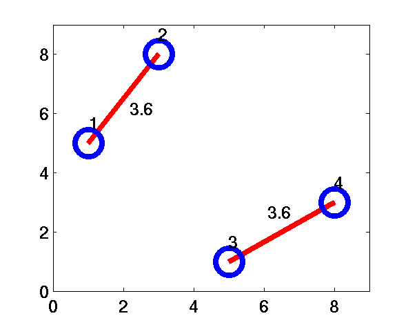
Figure 1 (a)

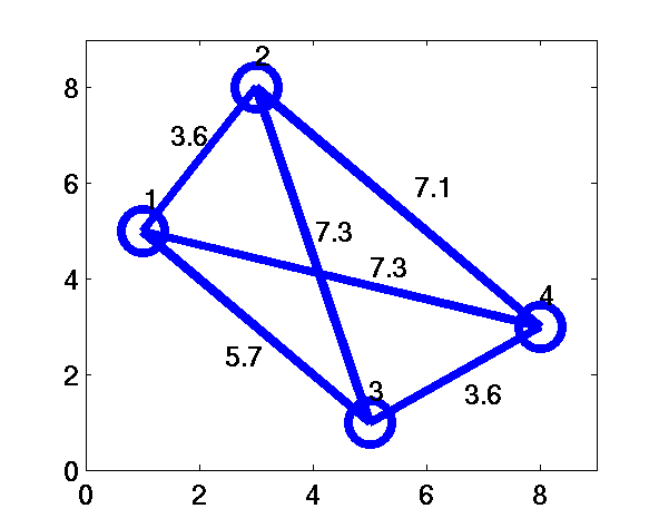
Figure 1 (b)

The possible pairing of points are given in Figures 2 (a) to 2 (c).

Figure 2 (a): L=7.2

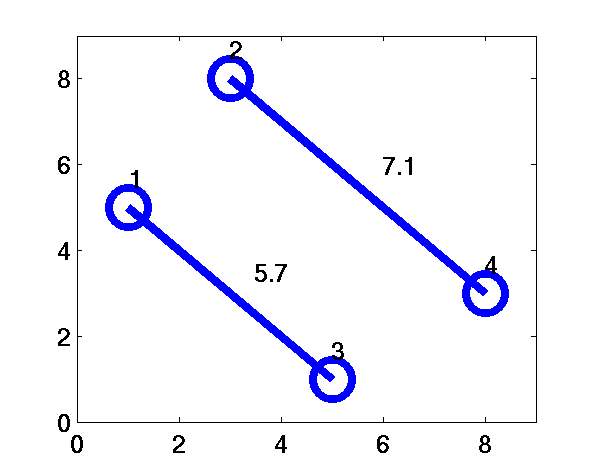
Figure 2 (b): L=12.8

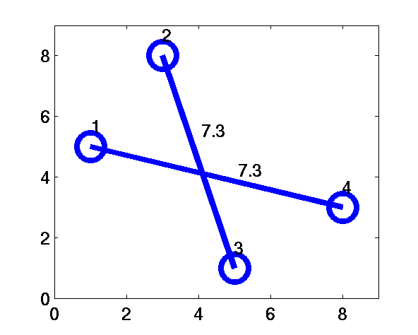
Figure 2 (c): L=14.6

The total length of the paired links (( L=\sum\limits_{i\lt j}d_{ij}n_{ij} )) are 7.2, 12.8 and 14.6, respectively.

Therefore, Fig.2a is the solution to this weighted matching problem.