a. Kalman Filter

The Kalman Filter algorithm is a powerful tool for estimating and predicting system states in the presence of uncertainty and is widely used as a fundamental component in applications such as target tracking, navigation, and control. The Kalman Filter predicts the future system state based on past estimations.

Kalman filter is an algorithm that combines information about the state of a system using predictions based on a physical model and noisy measurements. It is called a filter because it filters out measurement noise. Kalman filter has many applications in robotics. For example, it can be used for localization of coordinates and velocity of a robot based on measurements of distance to certain landmarks. It is widely used for filtering information from GPS sensors and radars.

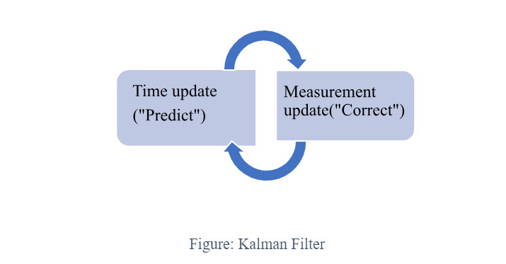
Kalman Filter performs two main operations:

1. Estimating the next state of the system
2. Correcting the estimated state with actual measurements

Kalman filters combine predicted states and noisy measurements to produce optimal, unbiased state estimates. The initial ensemble contains information about the initial states, parameters, and their uncertainties.

---

Kalman Filter Equations

The Kalman Filter maintains estimates of the state vector and the error covariance matrix.

Notations

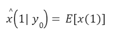
• X(t|t) — Estimate of x(t) given measurements z(t), z(t−1), …
• X(t+1|t) — Estimate of x(t+1) given measurements z(t), z(t−1), …
• P(t|t) — Covariance of X(t)
• P(t+1|t) — Covariance of X(t+1)
• H(t) — Transformation matrix
• G(t) — Kalman Gain

---

State Estimation

Known quantities are: x(t|t), u(t), P(t|t), and the new measurement z(t+1).

---

Time Update (Prediction Step)

1. State Prediction

x(t+1|t) = F(t)x(t|t) + G(t)u(t)

2. Measurement Prediction

z(t+1|t) = H(t)x(t+1|t)

---

Measurement Update (Correction Step)

1. Measurement Residual

w(t+1) = z(t+1) - z(t+1|t)

2. Updated State Estimate

x(t+1|t+1) = x(t+1|t) + W(t+1)w(t+1)

where W(t+1) is the Kalman Gain.

---

State Covariance Estimation

1. State Prediction Covariance

P(t+1|t) = F(t)P(t|t)F(t)' + Q(t)

2. Measurement Prediction Covariance

S(t+1) = H(t+1)P(t+1|t)H(t+1)' + R(t+1)

3. Kalman Gain

W(t+1) = P(t+1|t)H(t+1)'S(t+1)^{-1}

4. Updated State Covariance

P(t+1|t+1) = P(t+1|t) - W(t+1)S(t+1)W(t+1)'

---

b. Kalman Filter with Unforced Dynamic Model and Noiseless State-Space Representation

The Kalman filter is a recursive algorithm for estimating the state of a linear dynamic system from noisy observations.

This section describes a specialized form of the Kalman filter applied to an unforced dynamic model with a noiseless state-space representation (no process noise), as introduced by Sayed and Kailath (1994).

This model is characterized by:

• Absence of process noise (Q = 0)
• Simplified scalar state transition governed by the forgetting factor λ

This particular formulation serves as a foundational framework for deriving the family of Recursive Least Squares (RLS) adaptive filtering algorithms.

State-Space Model

The linear dynamical system is described by the following equations:

1. State Equation (unforced, no process noise):

   x(n+1) = λ^(-1/2) x(n)

   where λ is a positive real scalar (forgetting factor, 0 < λ ≤ 1).

2. Measurement Equation:

   y(n) = u^H(n) x(n) + v(n)

   where:

   • u(n) is the regressor (input) vector
   • v(n) is scalar zero-mean white measurement noise with unit variance:

Key Characteristics

• Unforced dynamics: No process noise → state evolves deterministically
• Measurement noise: v(n) is zero-mean white noise with variance 1
• State transition: Scalar multiplier λ^(-1/2) instead of a full matrix

Initial Conditions

• Initial state estimate:

• Initial error covariance:

Kalman Filter Equations for This Model

1. Time Update (Prediction Step)

State prediction (from time n−1 to n):

Predicted error covariance:

2. Measurement Update (Correction Step)

• Kalman Gain:

• Measurement residual (innovation):

• Updated state estimate:

• Updated error covariance:

Significance

This simplified Kalman filter formulation — with no process noise and scalar state transition — provides a clean mathematical bridge to understanding the Recursive Least Squares (RLS) algorithm family.

The scalar forgetting factor λ plays a central role, controlling the memory depth and tracking capability of the filter. This approach enables efficient and accurate state estimation in the presence of measurement noise only, and forms the theoretical basis for many modern adaptive filtering techniques used in signal processing, system identification, and equalization.