
Compare the Frequency Responses using Different Methods and Sampling Times 
Procedure
Steps to perform the simulation
- At first enter the coefficient values of the transfer function and sampling time T.
- Click on 'G(s)' button to get the partial fraction form of the transfer function.
- Click on 'Discretization' dropdown-menu to get different methods.
- Click on the desired option to select the discrete form of the system.
- Click on the 'Run' button option to get the selected discrete form of the system.
- Results of the discretized form will be displayed for the selected method.
- Results of the discretized form: Transfer Function and Frequency Transfer Function by Impulse Invariance Method.
- Results of the discretized form: Transfer Function and Frequency Transfer Function by Bilinear Transformation Method.
- Click on 'Frequency Response Plot' button to get the desired frequecy response plot.
- Click on 'Clear' button to get results for new transfer function.
- Click on 'Download Plot' button to download the plot.
- Note: Run the methods for different sampling times sequentially without clicking 'Clear' button, then click 'Compare' button to compare the responses.
- Note: A maximum of six frequency response experiments can be conducted and plotted for comparison.
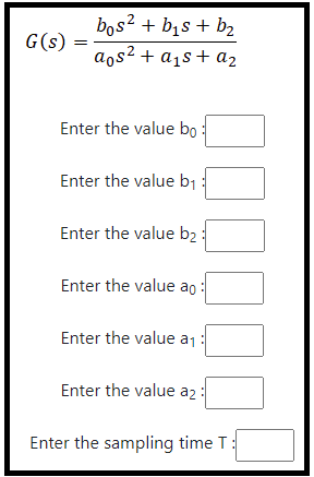
Fig. 1. Coefficient values entry for continuous transfer function

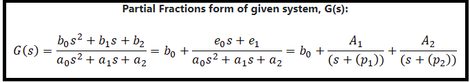
Fig. 2. Partial fraction form of continuous transfer function
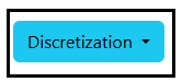
Fig. 3. Dropdown menu button to get different discretization methods
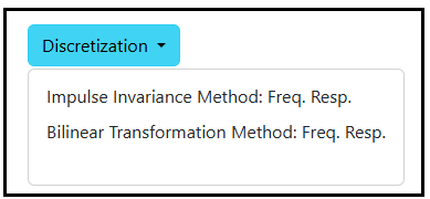
Fig. 4. Desired option to select the discrete form
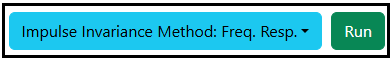
Fig. 5. Run button to get the selected discrete form

Fig. 6. Discretization form by Impulse Invariance Method
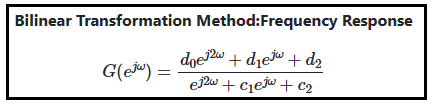
Fig. 7. Discretization form of Bilinear Transformation Method

Fig. 8. Button to get the desired plot