
Quantum Mechanics of the Hydrogen Atom
Part 1: Understanding the Interface
- Begin the Simulation - Access the Hydrogen Orbital Visualizer in your web browser
- Familiarize with Controls:
- Principal Quantum Number (n): Slider from 1 to 7
- Azimuthal Quantum Number (ℓ): Slider from 0 to (n-1)
- Magnetic Quantum Number (mₗ): Slider from -ℓ to +ℓ
- Identify Display Sections:
- Left Panel: Quantum Controls and Preset Buttons
- Center: Orbital Visualization Canvas
- Right Panel: Orbital Information and Energy Display
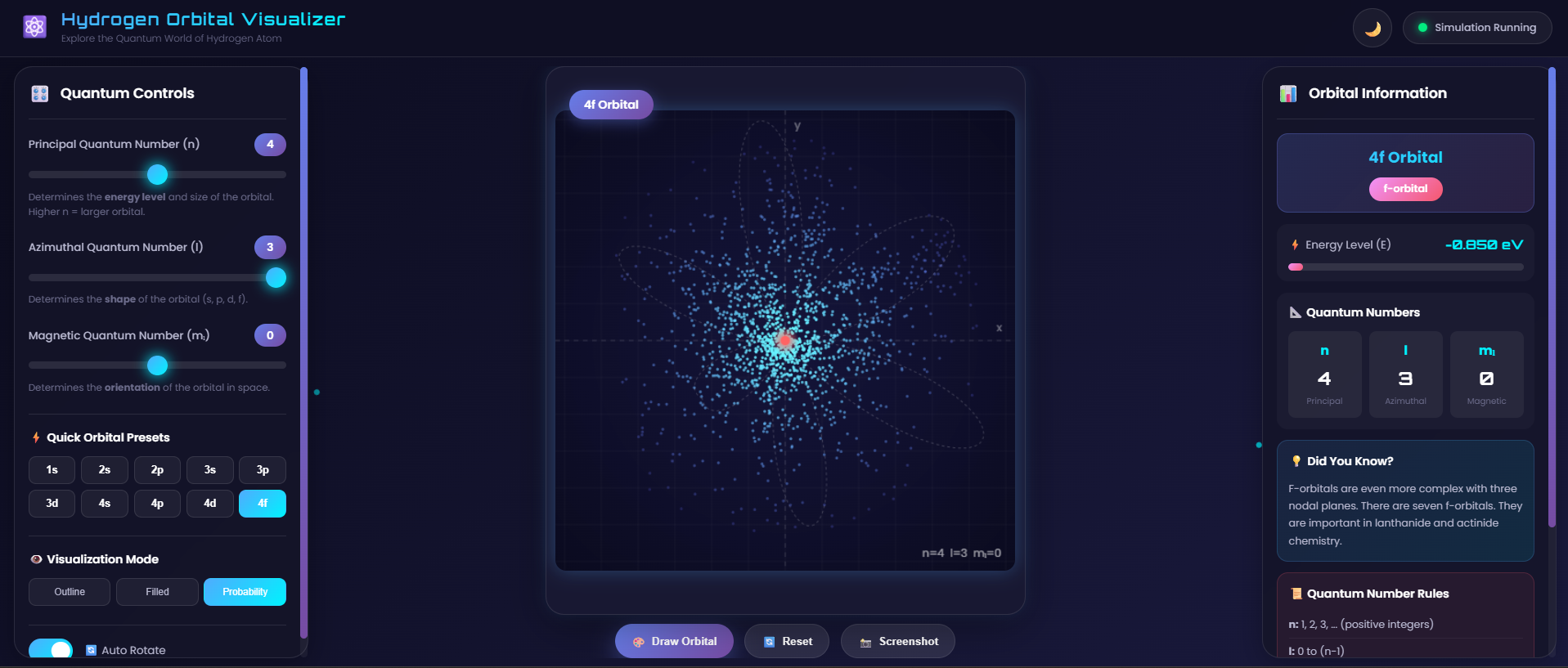
Fig. 1: Hydrogen Orbital Visualizer - Main Interface showing quantum controls, 3D visualization, and orbital information
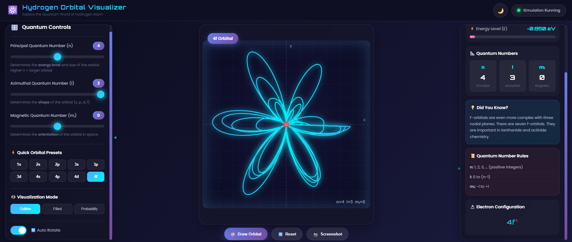
Fig. 2: Various orbital shapes (s, p, d, f) visualized in the simulation with different quantum number combinations
Part 2: Exploring s-Orbitals (ℓ = 0)
- Set n = 1, ℓ = 0, mₗ = 0 (1s orbital)
- Observe the spherical shape
- Note the energy value: -13.6 eV
- Set n = 2, ℓ = 0, mₗ = 0 (2s orbital)
- Compare size with 1s orbital
- Record your observations below
Part 3: Exploring p-Orbitals (ℓ = 1)
- Set n = 2, ℓ = 1, mₗ = 0 (2p orbital)
- Observe the dumbbell shape
- Change mₗ to -1 and +1, note orientation changes
- Repeat for n = 3 (3p orbitals)
- Compare energies across different p-orbitals
Part 4: Exploring d-Orbitals (ℓ = 2)
- Set n = 3, ℓ = 2, mₗ = 0 (3d orbital)
- Observe the cloverleaf pattern
- Vary mₗ from -2 to +2
- Note the five different d-orbital orientations
Part 5: Exploring f-Orbitals (ℓ = 3)
- Set n = 4, ℓ = 3, mₗ = 0 (4f orbital)
- Observe the complex multi-lobed structure
- Vary mₗ and observe all seven f-orbital shapes
Observation Table
Record your observations in the following table:
| S.No. | Orbital | n | ℓ | mₗ | Energy (eV) | Shape Observed |
|---|---|---|---|---|---|---|
| 1 | 1s | 1 | 0 | 0 | -13.6 | Spherical |
| 2 | 2s | 2 | 0 | 0 | -3.4 | Spherical (larger) |
| 3 | 2p | 2 | 1 | 0 | -3.4 | Dumbbell |
| 4 | 3s | 3 | 0 | 0 | -1.51 | Spherical (largest) |
| 5 | 3p | 3 | 1 | 0 | -1.51 | Dumbbell (larger) |
| 6 | 3d | 3 | 2 | 0 | -1.51 | Four-lobed cloverleaf |
| 7 | 4s | 4 | 0 | 0 | -0.85 | Spherical (very large) |
| 8 | 4f | 4 | 3 | 0 | -0.85 | Complex multi-lobed |
Visualization Modes
Use different visualization modes to understand orbital properties:
| Mode | Description | Best For |
|---|---|---|
| Outline | Shows orbital boundary | Understanding shape and symmetry |
| Filled | Shows solid orbital region | Visualizing 3D volume |
| Probability | Shows electron density distribution | Understanding probability density |
Analysis Questions
After completing the observations, answer the following:
- How does the orbital size change as n increases?
- What is the relationship between ℓ and orbital shape?
- How does the magnetic quantum number (mₗ) affect the orbital orientation?
- Why does energy become less negative as n increases?
- How many nodal surfaces do you observe in each orbital type?
Precautions
- Ensure valid quantum number combinations (ℓ < n, |mₗ| ≤ ℓ)
- Use the Reset button if visualization appears incorrect
- Allow animation to complete before changing parameters
- Take screenshots for documentation using the Screenshot button
Conclusion
Based on your observations, write a brief conclusion about:
- The relationship between quantum numbers and orbital properties
- How the visualization helps understand atomic structure
- The significance of probability density in quantum mechanics