Procedure

For Doing Simulation

1. Move the slider in Calibrate Telescope and click the START button.
2. Click on the combo box to select the lamp.
3. Click Switch On Light.
4. Set Vernier reading to 0° and telescope to 90° by adjusting both sliders.
5. Click the Place Grating button.
6. Turn the telescope to the left. Align the vertical cross wire with the green line on the pattern.
7. Note the readings of Vernier 1 and Vernier 2.
8. Move the telescope to the right side of the direct image and align the vertical cross wire with the green line on the pattern.
9. Note the readings of Vernier 1 and Vernier 2 again.
10. Use the slider under Fine Angle to get more precise readings.
11. Calculate the difference between the two readings on the same Vernier.
12. Take the mean value of this difference to get 2θ, twice the angle of diffraction. From this, θ is obtained for the green line.
13. Assuming the wavelength of the green line is 546 nm, calculate the number of lines per mm using the equation: N = sinθ / (mλ) where m is the order.

For Doing the Real Lab

Setting the Grating for Normal Incidence Position

1. Fix the Vernier table after making the preliminary adjustments.
2. Illuminate the slit with a mercury vapour lamp and make the slit narrow.
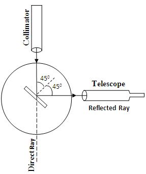
3. Bring the telescope in line with the collimator. Align the direct image of the slit with the vertical cross wire.
4. Note down any one of the Vernier readings.
5. Turn the telescope exactly through 90° and clamp it.
6. Place the grating on the prism table with its ruled surface facing the collimator and perpendicular to the line joining the two leveling screws of the prism table.
7. Unclamp the Vernier and rotate until the reflected image coincides with the vertical cross wire.
8. Fix the prism table and note the Vernier readings.
9. Unclamp the Vernier table and rotate exactly 45° in the proper direction so that the surface of the grating becomes normal to the collimator.
10. Clamp the Vernier table.

Standardizing the Grating

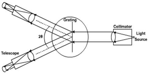
1. Move the telescope to observe the direct image. Diffraction patterns will be seen on either side of the direct image.
2. Turn the telescope to the left and align the vertical cross wire with the green line on the pattern.
3. Note the readings of Vernier 1 and Vernier 2.
4. Move the telescope to the right side of the direct image and align the vertical cross wire with the green line on the pattern.
5. Note the readings of Vernier 1 and Vernier 2 again.
6. Calculate the difference between the two readings on the same Vernier.
7. Take the mean value of this difference to get 2θ. From this, calculate θ for the green line.
8. Assuming the wavelength of the green line is 546 nm, calculate the number of lines per mm using the equation: N = sinθ / (mλ).

To Determine the Wavelength of Other Lines

Repeat the same procedure as above for other lines, and calculate their wavelengths using the equation:

λ = sinθ / (N × m)

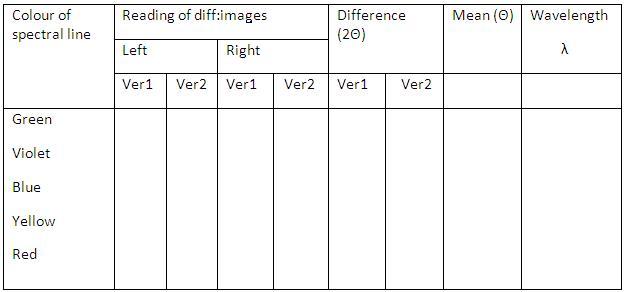
Results

The wavelength of the prominent lines of the mercury spectrum are given in nanometre in the tabular column.

Number of grating per metre=................/m