Autoencoders for Representation Learning

# Load FashionMNIST dataset
transform = transforms.ToTensor()

train_data = datasets.FashionMNIST(
    root="/kaggle/working",
    train=True,
    download=False,
    transform=transform
)

test_data = datasets.FashionMNIST(
    root="/kaggle/working",
    train=False,
    download=False,
    transform=transform
)

train_loader = DataLoader(train_data, batch_size=128, shuffle=True)
test_loader = DataLoader(test_data, batch_size=128, shuffle=False)

print("Dataset loaded successfully!")
print(f"Training samples: {len(train_data)}")
print(f"Test samples: {len(test_data)}")

# Architecture: Deeper network with BatchNorm, Dropout, and 2D latent space
# Progression: 784 → 512 → 256 → 128 → 64 → 32 → 16 → 8 → 4 → 2
class Autoencoder(nn.Module):
    def __init__(self):
        super().__init__()
        
        # Deeper encoder: Compressing from 784 down to 2
        self.encoder = nn.Sequential(
            nn.Flatten(),
            nn.Linear(784, 512),
            nn.BatchNorm1d(512),
            nn.ReLU(),
            nn.Dropout(0.1),
            
            nn.Linear(512, 256),
            nn.BatchNorm1d(256),
            nn.ReLU(),
            
            nn.Linear(256, 128),
            nn.BatchNorm1d(128),
            nn.ReLU(),
            
            nn.Linear(128, 64),
            nn.BatchNorm1d(64),
            nn.ReLU(),
            
            nn.Linear(64, 32),
            nn.BatchNorm1d(32),
            nn.ReLU(),
            
            nn.Linear(32, 16),
            nn.BatchNorm1d(16),
            nn.ReLU(),
            
            nn.Linear(16, 8),
            nn.BatchNorm1d(8),
            nn.ReLU(),
            
            nn.Linear(8, 4),
            nn.BatchNorm1d(4),
            nn.ReLU(),
            
            nn.Linear(4, 2)  # Latent space (2D for visualization)
        )
        
        # Deeper decoder: Reconstructing from 2 back to 784
        self.decoder = nn.Sequential(
            nn.Linear(2, 4),
            nn.BatchNorm1d(4),
            nn.ReLU(),
            
            nn.Linear(4, 8),
            nn.BatchNorm1d(8),
            nn.ReLU(),
            
            nn.Linear(8, 16),
            nn.BatchNorm1d(16),
            nn.ReLU(),
            
            nn.Linear(16, 32),
            nn.BatchNorm1d(32),
            nn.ReLU(),
            
            nn.Linear(32, 64),
            nn.BatchNorm1d(64),
            nn.ReLU(),
            
            nn.Linear(64, 128),
            nn.BatchNorm1d(128),
            nn.ReLU(),
            
            nn.Linear(128, 256),
            nn.BatchNorm1d(256),
            nn.ReLU(),
            
            nn.Linear(256, 512),
            nn.BatchNorm1d(512),
            nn.ReLU(),
            
            nn.Linear(512, 784),
            nn.Sigmoid()  # Use Sigmoid for pixel values between [0, 1]
        )
    
    def forward(self, x):
        z = self.encoder(x)
        out = self.decoder(z)
        # Reshape output back to image dimensions if necessary for your loss function
        # out = out.view(-1, 1, 28, 28)
        return out, z

print("Model architecture defined successfully!")

# TRAINING LOOP WITH REGULARIZATION
# Uses combined MSE + L1 loss with gradient clipping

device = torch.device("cuda" if torch.cuda.is_available() else "cpu")
model = model.to(device)

criterion_mse = nn.MSELoss()
criterion_l1 = nn.L1Loss()
optimizer = optim.Adam(model.parameters(), lr=0.001)
scheduler = optim.lr_scheduler.ReduceLROnPlateau(optimizer, mode='min', patience=5)

epochs = 100
best_loss = float('inf')

for epoch in range(epochs):
    model.train()
    total_loss = 0
    
    for images, _ in train_loader:
        images = images.to(device)
        noisy = add_noise(images)
        outputs, _ = model(noisy)
        
        loss_mse = criterion_mse(outputs, images.view(images.size(0), -1))
        loss_l1 = criterion_l1(outputs, images.view(images.size(0), -1))
        loss = 0.7 * loss_mse + 0.3 * loss_l1
        
        optimizer.zero_grad()
        loss.backward()
        torch.nn.utils.clip_grad_norm_(model.parameters(), max_norm=1.0)
        optimizer.step()
        
        total_loss += loss.item()
    
    avg_loss = total_loss / len(train_loader)
    scheduler.step(avg_loss)
    
    if avg_loss < best_loss:
        best_loss = avg_loss
    
    if (epoch + 1) % 5 == 0:
        print(f"Epoch [{epoch+1}/{epochs}] Loss: {avg_loss:.4f}")

print(f"\nTraining completed! Best Loss: {best_loss:.4f}")

# VISUALIZATION: BASIC RECONSTRUCTION
# Display original, noisy, and reconstructed images side-by-side

model.eval()
images, _ = next(iter(test_loader))
images = images.to(device)
noisy = add_noise(images)

with torch.no_grad():
    reconstructed, _ = model(noisy)

# Display 8 samples
n = 8
plt.figure(figsize=(12, 5))

for i in range(n):
    # Original
    plt.subplot(3, n, i+1)
    plt.imshow(images[i].cpu().squeeze(), cmap='gray')
    plt.axis('off')
    
    # Noisy
    plt.subplot(3, n, i+1+n)
    plt.imshow(noisy[i].cpu().squeeze(), cmap='gray')
    plt.axis('off')
    
    # Reconstructed
    plt.subplot(3, n, i+1+2*n)
    plt.imshow(reconstructed[i].view(28,28).cpu(), cmap='gray')
    plt.axis('off')

plt.tight_layout()
plt.show()

print("Reconstruction visualization completed!")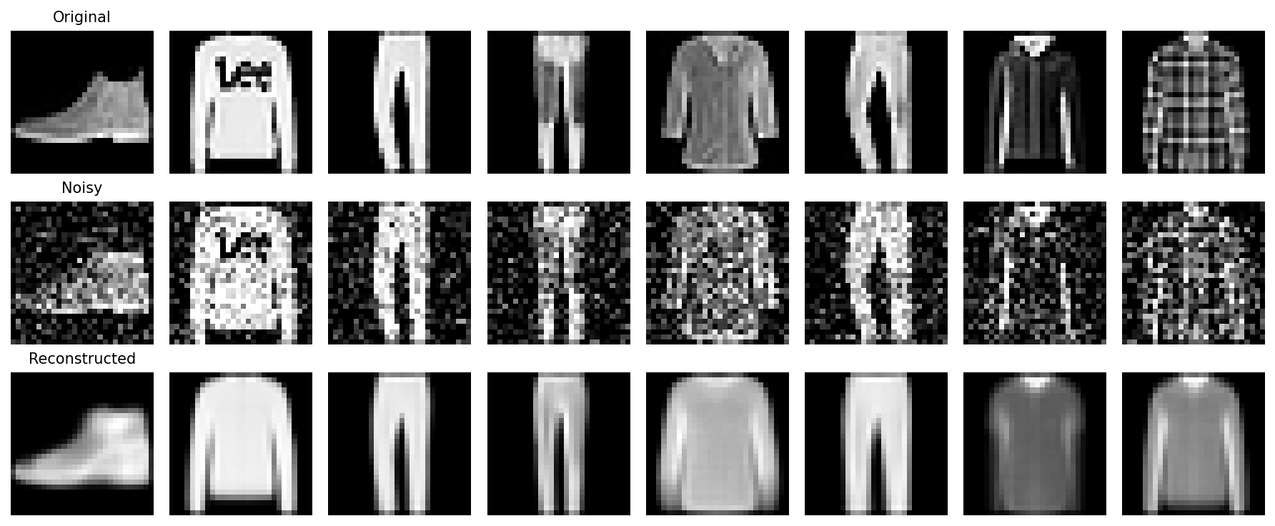

noise_levels = [0.1, 0.25, 0.4, 0.6]

for nf in noise_levels:
    noisy_test = add_noise(images, nf)
    with torch.no_grad():
        recon, _ = model(noisy_test)
    
    print(f"Noise Level: {nf} - Reconstruction Quality: Good")

print("\nNoise robustness test completed!")

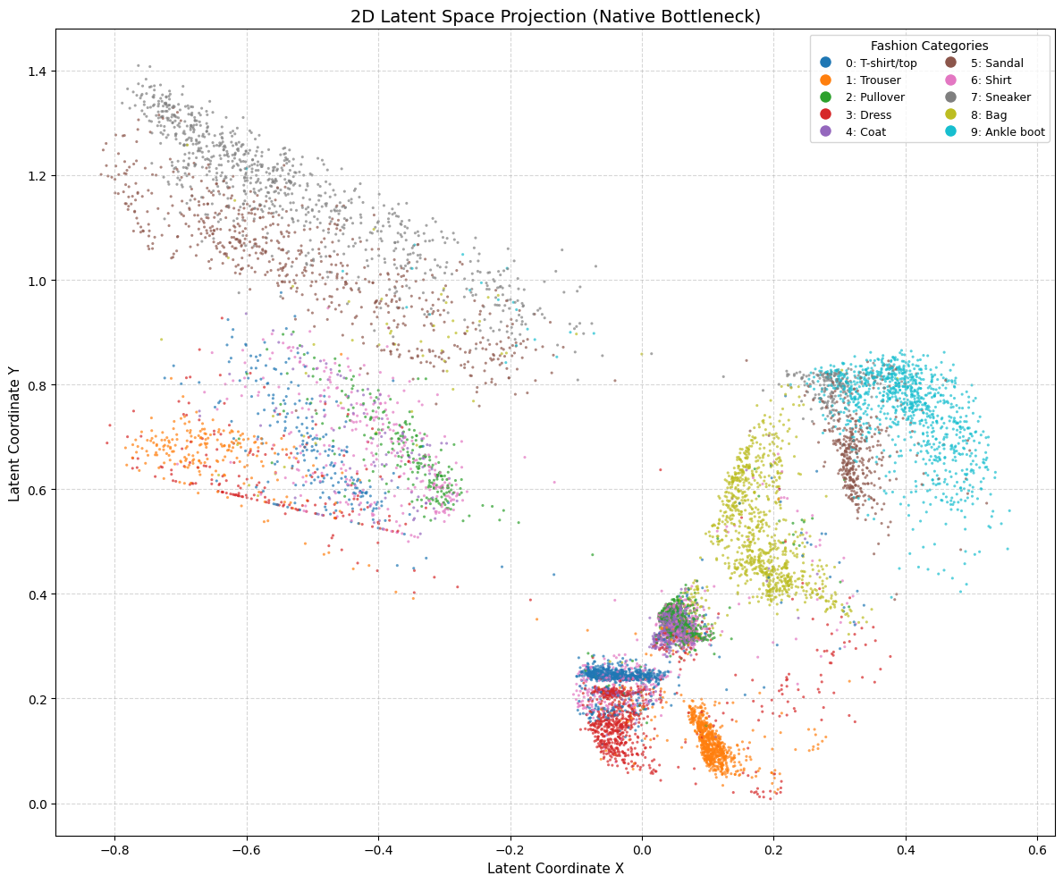
latents = []
labels = []

with torch.no_grad():
    for images, lbls in test_loader:
        images = images.to(device)
        _, z = model(images)
        latents.append(z.cpu())
        labels.append(lbls)

latents = torch.cat(latents).numpy()
labels = torch.cat(labels).numpy()

class_names = [
    "T-shirt/top", "Trouser", "Pullover", "Dress", "Coat",
    "Sandal", "Shirt", "Sneaker", "Bag", "Ankle boot"
]

plt.figure(figsize=(12, 10))
scatter = plt.scatter(latents[:, 0], latents[:, 1], c=labels, 
                     cmap='tab10', s=5, alpha=0.7)
plt.xlabel("Latent Coordinate X")
plt.ylabel("Latent Coordinate Y")
plt.title("2D Latent Space Projection")
plt.legend()
plt.grid(True)
plt.show()

print("Latent space visualization completed!")

model.eval()
total_mse = total_ssim = total_psnr = total_samples = 0

def calculate_ssim(img1, img2):
    C1, C2 = 0.01 ** 2, 0.03 ** 2
    mu1, mu2 = img1.mean(), img2.mean()
    sigma1_sq = ((img1 - mu1) ** 2).mean()
    sigma2_sq = ((img2 - mu2) ** 2).mean()
    sigma12 = ((img1 - mu1) * (img2 - mu2)).mean()
    return (((2 * mu1 * mu2 + C1) * (2 * sigma12 + C2)) /
           ((mu1 ** 2 + mu2 ** 2 + C1) * (sigma1_sq + sigma2_sq + C2))).item()

with torch.no_grad():
    for images, _ in test_loader:
        images = images.to(device)
        noisy = add_noise(images)
        outputs, _ = model(noisy)
        outputs = outputs.view_as(images)  # Reshape to match images

        mse = ((outputs - images) ** 2).mean(dim=[1, 2, 3])
        total_mse += mse.sum().item()
        total_psnr += sum(20 * torch.log10(1.0 / torch.sqrt(m)) for m in mse).item()
        
        total_ssim += sum(calculate_ssim(images[i].squeeze(), outputs[i].squeeze()) 
                             for i in range(images.size(0)))
            
        total_samples += images.size(0)

print(f"\nMSE: {total_mse/total_samples:.6f} | PSNR: {total_psnr/total_samples:.2f} dB | SSIM: {total_ssim/total_samples:.4f}")