A.Minimum Variance Distortion less Beamformer Using LMS and Monte-Carlo Runs

Introduction to Beamforming

Beamforming is a signal processing technique used in sensor arrays for directional signal transmission or reception. This technique involves combining signals from multiple sensors in such a way that signals from a particular direction are constructively combined while those from other directions are destructively interfered. Beamforming is widely used in applications such as radar, sonar, wireless communications, and audio signal processing.

Minimum Variance Distortion less Response (MVDR) Beamformer

The MVDR beamformer, also known as the Capon beamformer, is designed to minimize the output power of the beamformer subject to the constraint that the response in the direction of the desired signal remains unity. This can be mathematically expressed as:
min_ww^HHRw subject to w^Ha(θ) = 1
where:
w is the beamforming weight vector,
R is the covariance matrix of the input data,
a(θ) is the steering vector in the direction θ
The solution to this optimization problem is given by:
w_MvDR =R^-1-a(θ)/aHR-1a(θ)
This solution ensures that the desired signal is preserved while minimizing the power from interference and noise.

Least Mean Squares (LMS) Algorithm

The Least Mean Squares (LMS) algorithm is an adaptive filter used to find the filter coefficients that minimize the mean square error between the desired signal and the actual output of the filter. In the context of beamforming, the LMS algorithm can be used to iteratively adjust the beamforming weights to minimize the output power. The update rule for the weights is given by:
w(n + 1) = w(n) - μx(n)ⅇ*(n)
where:
μ is the step size parameter,
x(n) is the input signal vector at time n,
e(n) is the error signal, defined as the difference between the desired signal and the actual output.
The LMS algorithm is simple to implement and computationally efficient, making it suitable for real-time applications.

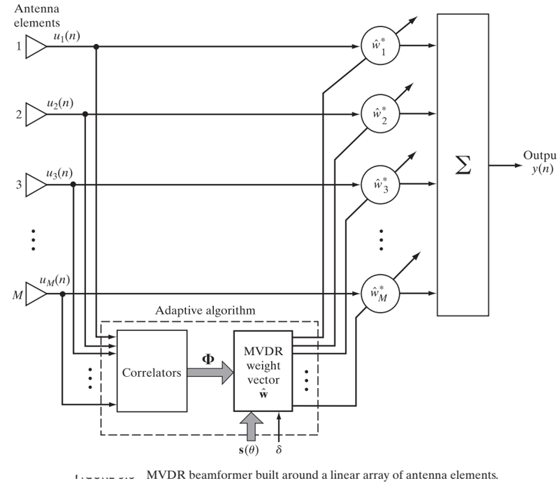
Figure 1.1

Monte Carlo Simulations

Monte Carlo simulations are a statistical technique used to model and analyse the behaviour of complex systems through random sampling. In the context of beamforming, Monte Carlo simulations can be used to evaluate the performance of the MVDR beamformer under various scenarios, such as different signal-to-noise ratios, array geometries, and interference conditions.
The combination of MVDR beamforming with the LMS algorithm and Monte Carlo simulations provides a robust framework for adaptive beamforming. The LMS algorithm adapts the beamforming weights in real-time, ensuring that the MVDR criterion is satisfied even in changing environments. Monte Carlo simulations can be used to evaluate the performance of this adaptive approach under different scenarios and validate its effectiveness.

Advantages

• Real-Time Adaptation:
  The LMS algorithm allows for real-time adjustment of the beamforming weights, making the system adaptable to changing conditions.

• Performance Evaluation:
  Monte Carlo simulations provide a comprehensive evaluation of the system's performance under various scenarios, ensuring robustness.

  Disadvantages

• Computational Complexity:
  While the LMS algorithm is computationally efficient, the overall complexity can increase with the size of the sensor array and the number of Monte Carlo runs.

• Convergence:
  Ensuring convergence of the LMS algorithm to the optimal solution requires careful selection of the step-size parameter μ.

  AR process with LMS and monte-carlo runs

  Autoregressive models operate under the premise that past values have an effect on current values, which makes the statistical technique popular for analysing nature, economics, and other processes that vary over time. Multiple regression models forecast a variable using a linear combination of predictors, whereas autoregressive models use a combination of past values of the variable.

Figure 1.2 We consider the example of M order AR process that is real valued. The above figure shows the block diagram of model used to generate this process. Its time domain description is governed by the M order difference equation
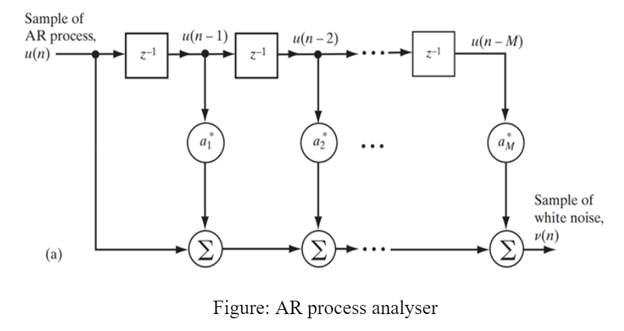
u(n)+a₁u(n-1)+a₂u(n-2)+...........+a₃u(n-M)=v(n) where v(n) is drawn from a white noise process of zero mean and variance σ².
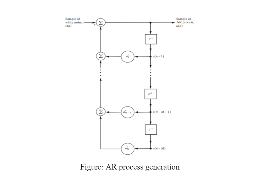
Figure 1.3 We use the error e(n) between the desired response d(n) and the output of the filter y(n) to tune the weights of the filter. The Least Mean Squares (LMS) algorithm is the most popular adaptive algorithm due to its simplicity and robustness.
The LMS algorithm performs the following operations to update the coefficients of an adaptive FIR filter:
1. Calculates the output signal y(n) from the FIR filter.
    y(n) = w^T(n)u(n)

    where u(n) is the tap-input vector at time n, defined by
    u(n) = [u(n), u(n-1), ..., u(n-M+1)]^T,

    and w(n) is the tap-weight vector at time n, defined by
    w(n) = [w₀(n), w₁(n), ..., w_M-1(n)]^T

2. Calculates the error signal e(n) by using the following equation:
   

    e(n) = d(n) − y(n)

3. Updates the filter coefficients by using the following equation:
   

    w(n + 1) = w(n) + μu(n)e^*(n)

    where y(n) = w^T(n)u(n)

    where,
    μ is the step size of the adaptive filter
    w(n) is the filter coefficients vector
    u(n) is the filter input vector.

A Monte Carlo simulation is used to model the probability of different outcomes in a process that cannot easily be predicted due to the intervention of random variables. It is a technique used to understand the impact of risk and uncertainty. A Monte Carlo simulation is used to tackle a range of problems in many fields, including investing, business, physics, and engineering. It is also referred to as a multiple probability simulation.

The Monte Carlo simulation is a mathematical technique that predicts possible outcomes of an uncertain event. Monte Carlo simulation is a type of computational algorithm that uses repeated random sampling to obtain the likelihood of a range of results occurring.

B.Adaptive Prediction And Equalization Using Least Mean Squares (LMS) And Recursive Least Squares (RLS) Algorithms.

Adaptive Equalization

In adaptive equalization, the filters adopt themselves to the dispersive effects of the channel. An adaptive equalizer automatically adapts to time-varying properties of the communication channel. The technique of equalization is used to reduce the additive noise. These equalizers are majorly kept in the receiver side. The theory behind this is that the filter characteristics should be optimized. The filter coefficients of an adaptive filter are based on error signal e(n) between the filter output d̂(n) and desired signal d(n).Goal of equalizers is to overcome the negative effects of the channel.

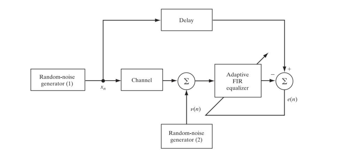
Figure 1.4

Adaptive equalization using LMS

Least mean squares (LMS) algorithms are a class of adaptive filter used to mimic a desired filter by finding the filter coefficients that relate to producing the least mean squares of the error signal (difference between the desired and the actual signal). It is a stochastic gradient descent method in that the filter is only adapted based on the error at the current time. LMS filter is built around a transversal (i.e. tapped delay line) structure. Two practical features, simple to design, yet highly effective in performance have made it highly popular in various application. LMS filter employ, small step size statistical theory, which provides a fairly accurate description of the transient behaviour. It also includes H∞ theory which provides the mathematical basis for the deterministic robustness of the LMS filters. As mentioned before LMS algorithm is built around a transversal filter, which is responsible for performing the filtering process. A weight control mechanism responsible for performing the adaptive control process on the tape weight of the transversal filter. 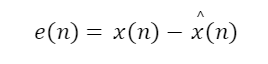The LMS algorithm in general, consists of two basics procedure: Filtering process, which involve, computing the output of a linear filter in response to the input signal and generating an estimation error by comparing this output with a desired response as follows:
e(n) = d(n) - y(n)
The LMS algorithm is based on minimizing the instantaneous error i.e. e²(n) with respect to the filter coefficient vector h(n). The filter weights are updated as:
w(n + 1) = w(n) + μe(n)y(n)

Adaptive equalization using RLS

RLS is advantageous in adaptive equalization for its ability to quickly adapt to channel variations. It provides a high level of performance in environments where the channel characteristics change rapidly, ensuring that the equalizer can effectively mitigate ISI and maintain signal integrity.

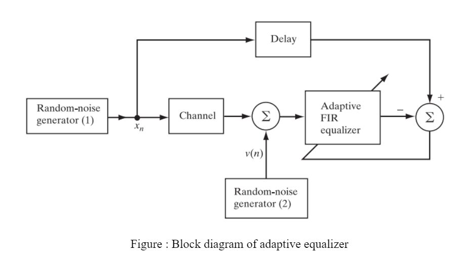
Figure 1.5

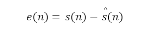
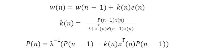
In adaptive equalization, the received signal y(n) is passed through an adaptive filter to produce the equalized output ŝ(n). The error signal e(n), which is the difference between the desired signal s(n) and the equalized output, guides the adaptation process:<

The RLS algorithm updates the filter coefficients wn to minimize the weighted sum of squared errors: The recursive update rules for RLS in the context of equalization are: where y(n) represents the input vector to the equalizer.
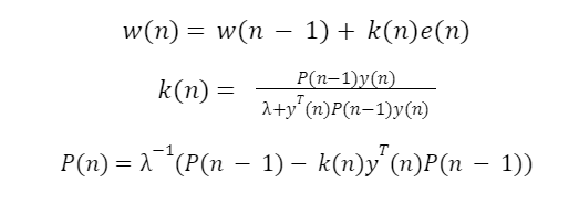
where P(n) is the inverse correlation matrix and k(n) is the gain vector.

Adaptive Prediction via LMS

Commonly used filters can be divided into three kinds: FIR (Finite Impulse Response) filter, IIR (Infinite Impulse Response) filter, and adaptive filter. The precondition of FIR filter and IIR filter is that the statistical characteristics of input signals are known. The premise design condition of adaptive filter is that some of the statistical characteristics of input signals are unknown. The performance indexes of filter can be replaced by the estimated value of unknown signal. In order to analyse the adaptive filter based on LMS (Least Mean Square) algorithm, the principle and application of adaptive filter should be introduced, and the simulation results based on the statistical experimental method are presented according to the principle and structure of LMS algorithm. The applications of adaptive filtering technology are shown by the introduction of three parts: an adaptive linear filter for the correction of channel mismatch, an adaptive equalizer for the improvement of system performance, and an adaptive notch filter for the elimination of the interference signal with known frequency.

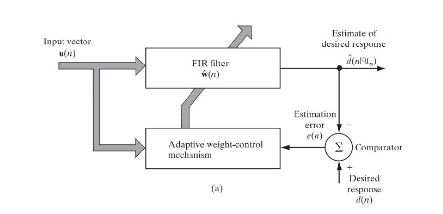
Figure 1.6 Desired output is generated as:
u(n) =- au(n - 1) + v(n)
where a = -0.98 and v(n) is gaussian white noise.
Hence the optimal value of estimated weight = a

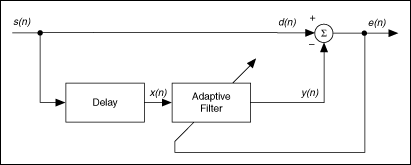
Figure 1.7 Predicting signals requires that you make some key assumptions. Assume that the signal is either steady or slowly varying over time, and periodic over time as well.
Accepting these assumptions, the adaptive filter must predict the future values of the desired signal based on past values. When s(n) is periodic and the filter is long enough to remember previous values, this structure with the delay in the input signal, can perform the prediction.

Adaptive Prediction via RLS

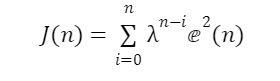
Adaptive prediction involves estimating future values of a signal based on past observations. This is critical in applications such as speech coding, echo cancellation, and financial time series forecasting. The goal is to minimize the prediction error, which is the difference between the actual signal and its predicted value. The RLS algorithm is preferred for adaptive prediction due to its recursive nature and rapid convergence. Unlike other algorithms such as the Least Mean Squares (LMS), RLS minimizes the weighted sum of squared errors with an exponential weighting factor, providing a robust and efficient means of updating prediction parameters.

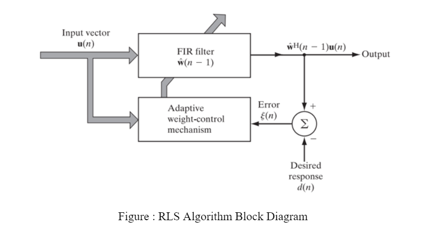
Figure 1.8 Given a discrete time signal x(n), the predicted value x̂(n+1) is based on a linear combination of past values x(n),x(n-1),…,x(n - p + 1). The prediction error e(n) is given by:

In the RLS algorithm, the coefficients wn are updated to minimize the cost function:

where 0 < λ ≤ 1 is the forgetting factor. The recursive update equations for the RLS algorithm are:
where P(n) is the inverse correlation matrix and k(n) is the gain vector.
The learning curve and random walk behavior are critical aspects of understanding and evaluating adaptive prediction and equalization algorithms. The LMS algorithm is characterized by its simplicity and slower convergence, as evidenced by its gradual learning curve and susceptibility to random walk behavior in noisy environments. In contrast, the RLS algorithm offers faster convergence and higher accuracy, with a sharp initial decline in its learning curve and reduced random walk behavior, making it more suitable for dynamic and high-performance applications.