Theory

Neural network learning is governed by the interaction between activation functions and optimization algorithms. Activation functions introduce non-linearity into the network, enabling it to learn complex input–output mappings, while optimization algorithms determine how model parameters are updated to minimize the loss function. The choice of activation function and optimizer significantly affects gradient propagation, convergence speed, training stability, and overall model performance. This experiment studies these effects using a Multilayer Perceptron trained on the Fashion-MNIST dataset.

2.1 Activation Functions

Activation functions are a fundamental component of artificial neural networks, as they introduce non-linearity into the model and enable learning of complex input–output relationships. In a Multilayer Perceptron (MLP), the activation function determines the output of a neuron based on the weighted sum of its inputs and bias. Without activation functions, even deep neural networks would behave like linear models and fail to capture complex patterns.

The choice of activation function significantly influences training dynamics, including gradient propagation, convergence speed, and stability during optimization. In this experiment, commonly used activation functions: Sigmoid, Hyperbolic Tangent (Tanh), and Rectified Linear Unit (ReLU) are employed in a Multilayer Perceptron (MLP) to analyse their effect on learning behaviour when trained on the Fashion-MNIST dataset.

Mathematical Formulation

Let the net input to a neuron be:

$$z = \sum_{i=1}^{n} w_i x_i + b$$

where $w_i$ represents weights, $x_i$ represents input features, and $b$ is the bias term. The output of the neuron is obtained by applying an activation function $f(z)$.

I. Sigmoid Activation Function: -

The sigmoid activation function is defined as:

$$\sigma(z) = \frac{1}{1 + e^{-z}}$$

The output of the sigmoid function lies in the range $(0, 1)$. It was commonly used in early neural networks due to its smooth and differentiable nature. However, for large positive or negative input values, the function saturates, resulting in very small gradients and slow convergence during training. The Figure 1 given below shows the behaviour of the Sigmoid activation function.

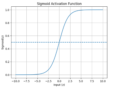
Figure 1: Sigmoid Activation Function

Merits of Sigmoid Activation Function

• Smooth and differentiable: The sigmoid function is continuously differentiable, which enables the use of gradient-based optimization techniques during training.
• Output in the range (0, 1): The output lies between 0 and 1, making it suitable for probability-based interpretation in binary classification problems.
• Simple mathematical formulation: The function is easy to understand and implement due to its straightforward mathematical expression.

Demerits of Sigmoid Activation Function

• Vanishing gradient problem: For large positive or negative input values, the gradients become extremely small, slowing down the learning process.
• Non-zero-centred output: The output is not zero-centred, which can cause inefficient weight updates and slower convergence during training.
• Saturation at extreme values: The function saturates at both ends of its output range, reducing its effectiveness in deep neural networks.

II. Hyperbolic Tangent (Tanh) Activation Function: -

The hyperbolic tangent activation function is given by:

$$\tanh(z) = \frac{e^z - e^{-z}}{e^z + e^{-z}}$$

The output range of tanh is $(-1, 1)$, making it zero-centred. Compared to sigmoid, tanh provides better gradient flow near zero and generally results in faster convergence. However, it still suffers from gradient saturation for large input values. The Figure 2 given below illustrates the behaviour of the Tanh activation function.

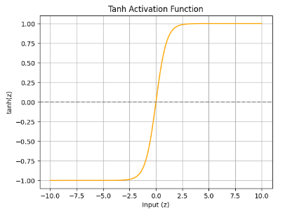
Figure 2: Tanh Activation Function

Merits of Hyperbolic Tangent (Tanh) Activation Function

• Zero-centred output: Helps improve gradient flow and speeds up convergence compared to sigmoid.
• Smooth and differentiable: The function supports stable gradient-based optimization due to its continuous differentiability.
• Stronger gradients near zero: Compared to sigmoid, tanh provides larger gradients around zero, which enhances learning efficiency.

Demerits of Hyperbolic Tangent (Tanh) Activation Function

• Vanishing gradient problem: Gradients become very small for large input values, which can slow down training in deeper networks.
• Saturation at extreme values: The function saturates at high positive and negative values, leading to reduced learning speed.
• Higher computational cost: The use of exponential functions makes tanh computationally more expensive than ReLU.

III. Rectified Linear Unit (ReLU): -

The Rectified Linear Unit activation function is defined as:

$$ReLU(z) = \max(0, z)$$

It can also be expressed in piecewise form as:

$$ReLU(z) = \begin{cases} 0, & \text{if } z < 0 \\ z, & \text{if } z \ge 0 \end{cases}$$

ReLU outputs zero for negative input values and a linear output for positive values. This behaviour significantly reduces the vanishing gradient problem and improves training efficiency. Due to its simplicity and effectiveness, ReLU is widely used in modern deep learning models. The Figure 3 given below represents the ReLU activation function curve.

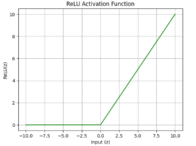
Figure 3: ReLU Activation Function

Merits of ReLU Activation Function

• Introduces non-linearity: ReLU enables neural networks to learn complex and non-linear relationships from data.
• Efficient training: Reduces vanishing gradient issues and accelerates convergence.
• Sparsity in activations: ReLU activates only a subset of neurons, improving computational efficiency and reducing overfitting.
• Simple and fast computation: The function involves only a threshold operation, making it computationally efficient.

Demerits of ReLU Activation Function

• Dying ReLU problem: Neurons can become inactive and permanently output zero, preventing further learning.
• Non-differentiable at zero: The function is not differentiable at zero, although this is handled using sub-gradients in practice.
• Unbounded output for positive inputs: The output for positive inputs is unbounded, which may lead to exploding activations if not properly controlled.

Comparison of Activation Functions

Activation Function	Mathematical Expression	Output Range	Merits	Demerits
Sigmoid	$\sigma(z) = \frac{1}{1 + e^{-z}}$	$(0, 1)$	Smooth and differentiable; suitable for probability-based outputs	Suffers from vanishing gradient and slow convergence
Tanh	$\tanh(z) = \frac{e^z - e^{-z}}{e^z + e^{-z}}$	$(-1, 1)$	Zero-centred output; better gradient flow than sigmoid	Vanishing gradient for large input values
ReLU	$ReLU(z) = \max(0, z)$	$[0, \infty)$	Fast convergence; reduces vanishing gradient problem	Dying ReLU problem; non-differentiable at zero

2.2 Optimization Algorithms

Optimization algorithms are used to minimize the loss function of a neural network by iteratively adjusting its parameters (weights and biases). During training, the optimizer determines the direction and magnitude of parameter updates based on the gradients of the loss function with respect to the model parameters. An efficient optimization algorithm ensures faster convergence, numerical stability, and improved generalization performance. In this experiment, Stochastic Gradient Descent (SGD) and Adaptive Moment Estimation (Adam) optimizers are studied and compared while training a Multilayer Perceptron (MLP) on the Fashion-MNIST dataset.

I. Stochastic Gradient Descent (SGD): -

Stochastic Gradient Descent is a fundamental optimization algorithm based on the theory of stochastic approximation, introduced by Herbert Robbins and Sutton Monro (1951). Unlike batch gradient descent, SGD updates model parameters using a single training example or a small mini-batch, which reduces computational cost.

The parameter update rule is:

$$\theta_{t+1} = \theta_t - \eta \nabla_\theta L(\theta_t)$$

where $\eta$ is the learning rate.

SGD is simple and memory-efficient, and the randomness in updates can help escape shallow local minima. However, it is sensitive to the learning rate and may converge slowly or exhibit oscillations during training.

Merits of Stochastic Gradient Descent (SGD)

• Simple and easy to implement: Stochastic Gradient Descent has a straightforward update rule, making it easy to understand and implement.
• Memory efficient: SGD requires very little additional memory, as it does not store past gradients or extra parameters.
• Ability to escape shallow local minima: The stochastic nature of parameter updates introduces noise, which can help the algorithm escape shallow local minima.
• Suitable for large datasets: SGD processes data in small batches, making it efficient for large-scale learning problems.

Demerits of Stochastic Gradient Descent (SGD)

• Sensitivity to learning rate: Choosing an inappropriate learning rate can result in slow convergence or unstable training.
• Slow convergence: SGD may require a large number of iterations to reach the optimal solution, especially for complex problems.
• No adaptive learning rate: A fixed learning rate is used for all parameters, which may limit performance if not carefully tuned.
• Oscillations during training: SGD can exhibit oscillatory behaviour near minima due to noisy gradient updates.

II. Adaptive Moment Estimation (Adam): -

Adaptive Moment Estimation (Adam) was proposed by Diederik P. Kingma and Jimmy Lei Ba (2015). It is an advanced optimization algorithm that combines the benefits of momentum-based methods and adaptive learning rate techniques. Adam adapts the learning rate for each parameter individually by maintaining exponentially decaying averages of past gradients and squared gradients.

The update rule for Adam is:

$$\theta_{t+1} = \theta_t - \eta \frac{\hat{m}_t}{\sqrt{\hat{v}_t} + \epsilon}$$

Where:

• $\theta_t$ is the model parameter at iteration $t$
• $\theta_{t+1}$ is the updated parameter
• $\eta$ is the learning rate
• $\hat{m}_t$ is the bias-corrected first moment estimate (mean of gradients)
• $\hat{v}_t$ is the bias-corrected second moment estimate (mean of squared gradients)
• $\epsilon$ is a small constant added for numerical stability

Adam provides faster convergence, stable training, and performs well with noisy or sparse gradients. Due to these advantages, it is widely used in deep learning applications.

Merits of Adaptive Moment Estimation (Adam)

• Adaptive learning rates: Adam automatically adjusts the learning rate for each parameter based on first and second moment estimates.
• Fast convergence: The optimizer converges faster than traditional gradient-based methods, especially on deep networks.
• Robust to noisy gradients: Adam performs well even when gradients are noisy or sparse.
• Minimal hyperparameter tuning: Default parameter values often work well, reducing the need for extensive tuning.

Demerits of Adaptive Moment Estimation (Adam)

• Higher computational cost: Adam requires additional computations to maintain moving averages of gradients and squared gradients.
• Increased memory usage: Extra memory is needed to store moment estimates for each parameter.
• Risk of overfitting: Adam may converge too aggressively, leading to overfitting on training data.
• Less theoretical convergence guarantees: Compared to SGD, Adam has weaker theoretical convergence properties in some cases.

Comparison of Optimization Algorithms

Optimization Algorithm	Learning Rate Type	Key Characteristics	Merits	Demerits
Stochastic Gradient Descent (SGD)	Fixed	Updates parameters using mini-batches	Simple, memory-efficient, good generalization	Sensitive to learning rate; slow convergence
Adaptive Moment Estimation (Adam)	Adaptive	Uses first and second moment estimates	Fast convergence; robust to noisy gradients	Higher computation and memory cost