Phase Modulation and Demodulation

Theory :

Phase modulation (PM) is a modulation technique where the phase of a carrier wave is varied according to the instantaneous amplitude of the modulating signal \( m(t) \). Unlike frequency modulation, where the frequency of the carrier is altered, in PM, the phase of the carrier signal is shifted. The modulated signal can be mathematically expressed as:

\( S(t) = A_c \cos\left[ 2\pi f_c t + K_p m(t) \right] \)

Where:

• \( A_c \) is the amplitude of the carrier signal.
• \( f_c \) is the carrier frequency.
• \( K_p \) is the phase sensitivity of the modulator, which determines how much the phase of the carrier is shifted in response to the modulating signal.
• \( m(t) \) is the modulating (baseband) signal.

In phase modulation, the phase of the carrier signal \( \cos\left[ 2\pi f_c t \right] \) is shifted by an amount proportional to the modulating signal \( m(t) \), scaled by the phase sensitivity \( K_p \). The amount of phase shift is directly proportional to the amplitude of the modulating signal.

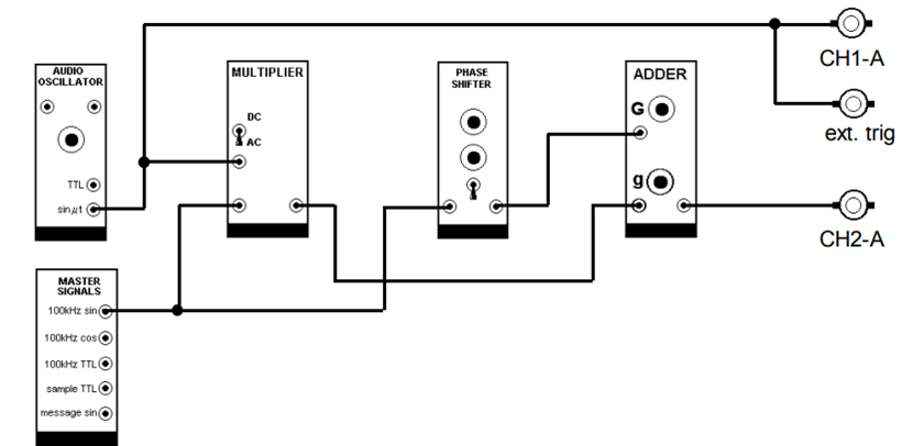
Figure 1

Armstrong's Phase Modulator

1. For amplitude modulation, defined as: AM = E.(1 + m.sinµt).sinωt …(i)
2. This expression can be expanded trigonometrically into the sum of two terms:
AM = E.sinωt + E.m.sinμt.sinωt …(ii)
3. In eqn.(ii) the two terms involved with 'ω' are in phase. Now this relation can easily be changed so that the two are at 90 degrees, or 'in quadrature'. This is done by changing one of the sinωt terms to cosωt. The signal then becomes what is sometimes called a quadrature modulated signal. It is Armstrong`s signal. Thus:
Armstrong`s signal = E.cosωt + E.m.sinμt.sinωt (iii)

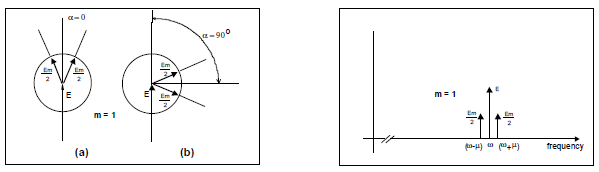
Fig 2: Phase modulation using DSBSC + carrier. (left) Phasor Diagram, (right) amplitude spectrum

Procedures

1. Choose a message frequency of about 1 kHz from the AUDIO OSCILLATOR
2. Check that the oscilloscope has triggered correctly, using the external trigger facility connected to the message source. Set the sweep speed so that it is displaying two or three periods of the message, on CH1-A, at the top of the screen
3. Rotate both g and G fully anti-clockwise.
4. Rotate g clockwise. Watch the trace on CH2-A. A DSBSC will appear. Increase its amplitude to about 3 volts peak-to-peak. Adjust the trace so its peaks just touch grid lines exactly a whole number of centimeters apart. This is for experimental convenience; it will be matched by a similar adjustment below.
5. Remove the patching cord from input g of the ADDER
6. Rotate G clockwise. The CARRIER will appear as a band across the screen. Increase its amplitude until its peaks touch the same grid lines as did the peaks of the DSBSC (the time base is too slow to give a hint of the fine detail of the CARRIER; in any case, the synchronization is not suitable).
7. Replace the patch cord to g of the ADDER. At the ADDER output there is now a DSBSC and a CARRIER, each of exactly the same peak-to-peak amplitude, but of unknown relative phase. Observe the envelope of this signal (CH2-A), and compare its shape with that of the message (CH1-A), also being displayed.
8. Vary the phasing with the front panel control on the PHASE SHIFTER until the almost sinusoidal envelope (CH2-A) is of twice the frequency as that of the message (CH1-A). The phase adjustment is complete when alternate envelope peaks are of the same amplitude.
9. Trim the front panel control of the PHASE SHIFTER until adjacent peaks of the envelope are of equal amplitude. To improve accuracy you can increase the sensitivity of the oscilloscope to display the peaks only. Equating heights of adjacent envelope peaks with the aid of an oscilloscope is an acceptable method of achieving the quadrature condition. For communication purposes the message distortion, as observed at the receiver, due to any such phase error, will be found to be negligible compared with the inherent distortion introduced by an ideal Armstrong modulator.
10. The envelope of Armstrong`s signal is recovered, using an envelope detector, and is monitored with a pair of headphones. For the in-phase condition this would be a pure tone at message frequency. As the phase is rotated towards the wanted 90 degrees difference it is very easy to detect, by ear, when the fundamental component disappears (at µ rad/s, and initially of large amplitude), leaving the component at 2µ rad/s, initially small, but now large. This is the quadrature condition.
11. Model an envelope detector, using the RECTIFIER in the UTILITIES module, and the 3 kHz LPF in the HEADPHONE AMPLIFIER module. Connect Armstrong`s signal to the input of the envelope detector. Listen to the filter output (the envelope) with headphones. Set the PHASE SHIFTER as far off the quadrature condition as possible, and concentrate your mind on the fundamental. Slowly vary the phase. You will hear the fundamental amplitude reduce to zero, while the second harmonic of the message appears. Notice how sensitive is the point at which the fundamental disappears ! This is the quadrature condition.
12. Set up for equal amplitudes of DSBSC and carrier into the ADDER of the modulator (β = 1), and confirm you have the quadrature condition. A message frequency of about 1 kHz will be convenient for spectral measurements
13. At the output of your Armstrong modulator add the AMPLITUDE LIMITER (the CLIPPER in the UTILITIES module) and filter (in the 100 kHz CHANNEL FILTERS module).
14. Model a WAVE ANALYSER, and connect it to the filter output. There is no need to calibrate it; you are interested in relative amplitudes.
15. Set the phase deviation to zero (by removing the DSBSC from the ADDER of the modulator). Observe and sketch the waveform of the signals into and out of the channel filter. Find the 100 kHz carrier component with the WAVE ANALYSER. This, the unmodulated carrier, is your reference. For convenience adjust the sensitivity of the SPECTRUM UTILITIES module so the meter reads full scale.
16. Replace the DSBSC to the ADDER of the modulator. The carrier amplitude should drop to 84% of the previous reading ,if you leave the meter switch on HOLD nothing will happen. Search for the first pair of sidebands. They should be at amplitudes of 38% of the unmodulated carrier.
17. There are further sideband pairs, but they are rather small, and will take care to find.
18. You could repeat the spectral measurements for β = 0.5 (which are also listed in Table A-1).
19. You were advised to look at the signal from the filter when there was no modulation. Do this again. Synchronize to the signal itself, and display ten or twenty periods. Then add the modulation. You will see the right hand end of the now modulated sine wave move in and out (the ‘oscillating spring’ analogy), confirming the presence of frequency modulation (there is no change to the amplitude).