Amplitude Modulation (AM)

Theory :

Amplitude modulation (AM) is the process in which the amplitude of a carrier wave, denoted as \( c(t) = \cos(2\pi f_c t) \), is varied in proportion to the baseband signal. This modulation technique can be mathematically represented as:

\( S(t) = A_c \left[ 1 + K_a m(t) \right] \cos(2\pi f_c t) \)

or equivalently,

\( S(t) = A_c \cos(2\pi f_c t) + A_c K_a m(t) \cos(2\pi f_c t) \)

where:

• \( K_a \) is the amplitude sensitivity of the modulator
• \( S(t) \) is the modulated signal
• \( A_c \) is the amplitude of the carrier signal
• \( m(t) \) is the modulating (baseband) signal

Modulation Index (μ) in Amplitude Modulation

The modulation index \( \mu \) quantifies the extent to which the carrier amplitude varies in response to the message signal.

It is commonly defined as:
\( \mu = K_a A_m \), where:

• \( A_m \) = peak amplitude of the message signal \( m(t) \)
• \( A_c \) = carrier amplitude
• \( K_a \) = amplitude sensitivity of the modulator

If \( K_a = 1 \), the expression simplifies to:
\( \mu = \frac{A_m}{A_c} \)

The value of \( \mu \) determines the modulation quality:

• \( \mu < 1 \): Under-modulation
• \( \mu = 1 \): 100% modulation (ideal)
• \( \mu > 1 \): Over-modulation (leads to distortion)

Alternative definition:
Even if \( K_a \) and \( A_m \) are unknown, the modulation index can be calculated directly from the modulated waveform:

\( \mu = \frac{A_{\text{max}} - A_{\text{min}}}{A_{\text{max}} + A_{\text{min}}} \)
where:

• \( A_{\text{max}} \) = maximum amplitude of the modulated signal
• \( A_{\text{min}} \) = minimum amplitude of the modulated signal

Power Efficiency and Distribution

A major topic in Amplitude Modulation (AM) is the analysis of how power is distributed within the transmitted signal. In the standard AM, a significant portion of the total transmitted power is concentrated in the carrier signal. Critically, this carrier wave itself conveys no information. The useful information—the original message signal—is contained entirely within the sidebands. The power efficiency (η) is a crucial metric that quantifies what fraction of the total power resides in these information-carrying sidebands.

• The efficiency is calculated using the formula:
  η = μ² / (2 + μ²)
  where μ represents the modulation index.
• Even under optimal conditions, such as 100% modulation (when μ=1), the maximum theoretical efficiency is only 33.3%. This means that a full two-thirds of the transmitter's power is expended just to send the carrier wave. This pronounced inefficiency is the primary motivation behind the development of more advanced, carrier-suppressed modulation techniques like Double-Sideband Suppressed-Carrier (DSB-SC) and Single-Sideband (SSB) modulation.

Bandwidth

While the provided lab text displays the spectrum of an AM signal, it does not explicitly state the formula for calculating its required bandwidth. The bandwidth is defined as the difference between the highest and lowest frequencies present in the modulated signal's spectrum.

• For a standard AM signal, the bandwidth is precisely twice the highest frequency component found in the modulating signal (also known as the message signal). The formula is:
  BW = 2 * f_m
  Where fm is the maximum frequency of the message signal.

APPARATUS :

1. TIMS-301 Modelling System
2. C.R.O (20MHz)
3. Spectrum Analyzer
4. Connecting chords & probes.

AM Signal, S(t) = E(1+m.cosμt) cosωt
Where, E is the amplitude of the AM signal
μ is the frequency of the message signal (in rad/s)
ω is the frequency of the carrier signal (in rad/s)
m is modulation index (varies from 0 to 1)

= {A(1+m.cosμt)} {B cosωt}
= {low frequency term a(t)} X {high frequency term c(t)}

The low frequency term can be considered as
a(t) = DC + m(t)
In the above equation with the help of adder we try to keep the modulation index or modulation depth exactly 100%

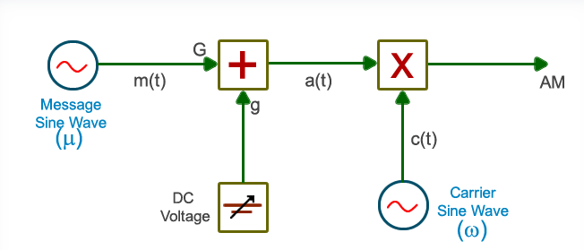
For example, if we set dc voltage at A volt and amplitude of the AC part of the above equation A.m, then their ratio is 1 at the output of the adder. Then 100% amplitude modulation is performed.

Circuit Diagram

Procedure for Amplitude Modulation

1. Generate a message signal from ‘AUDIO OSCILLATOR’ module as shown in the above. The AUDIO OSCILLATOR is a low distortion tuneable frequency sine wave source with a frequency range from 500Hz to 10kHz. Three outputs are provided. Two outputs are sinusoidal, with their signals in quadrature. The third output is a digital TTL level signal. Then pass the message signal thru the adder that can add a DC voltage and gain to the message signal.
The DC term comes from the VARIABLE DC module, and will be adjusted to the amplitude 'A' at the output of the ADDER.
The AC term m(t) will come from an AUDIO OSCILLATOR, and will be adjusted to the amplitude 'A•m' at the output of the ADDER. So that the modulation index, m be 1 or perfect AM modulation
a(t) = A(1+m.cosμt)
a(t) = DC + m(t)
a(t) = A + A.m.cosμt
So, m will be 1 as it is the ratio of A.m and A
2. Supply the 100 KHz carrier signal from the MASTER SIGNALS module
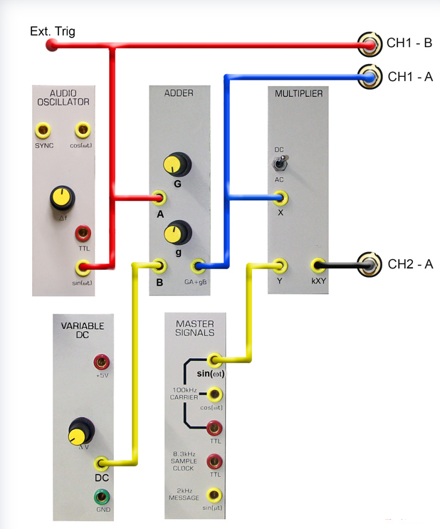
3. First patch up according to Figure above, but omit the input X and Y connections to the MULTIPLIER. Connect to the two oscilloscope channels using the SCOPE SELECTOR, as shown.
4. Use the FREQUENCY COUNTER to set the AUDIO OSCILLATOR to about 1 kHz.
5. Switch the SCOPE SELECTOR to CH1-B, and look at the message from the AUDIO OSCILLATOR. Adjust the oscilloscope to display two or three periods of the sine wave in the top half of the screen.
6. Now start adjustments by setting up a(t), and with m = 1
7. Turn both g and G fully anti-clockwise. This removes both the DC and the AC parts of the message from the output of the ADDER.
8. Switch the scope selector to CH1-A. This is the ADDER output. Switch the oscilloscope amplifier to respond to DC if not already so set, and the sensitivity to about 0.5 volt/cm.
9. Set gain on ADDER to set VDC
10. VDC = +1Volt
11. Now set amplitude of AC signal also to 1 Volt
12. Connect the output of the ADDER to input X of the MULTIPLIER. Make Sure the MULTIPLIER is switched to accept DC.
13. Now prepare the carrier signal:
c ( t ) = B.cosωt
14. Connect a 100 kHz analog signal from the MASTER SIGNALS module to input Y of the MULTIPLIER
15. Connect the output of the MULTIPLIER to the CH2-A of the SCOPE SELECTOR. Adjust the oscilloscope to display the signal conveniently on the screen.
16. Since each of the previous steps has been completed successfully, then at the MULTIPLIER output will be the 100% modulated AM signal. It will be displayed on CH2-A. It will look like this.

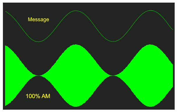
Fig: AM, with m=1

The percentage modulation can also be calculated from the modulated signal using the formula.
Percentage modulation = (Vmax-Vmin )/(Vmax +Vmin) × 100
Modulation factor = (Vmax-Vmin )/(Vmax +Vmin)

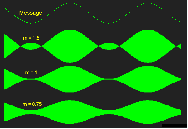
17. Vary the ADDER gain G, and thus 'm' and confirm that the envelope of the AM behaves as expected, including for values of m > 1.

Spectrum :

Analysis shows that the sidebands of the AM, when derived from a message of frequency μ rad/s, are located either side of the carrier frequency, spaced from it by μ rad/s

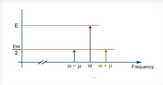
Fig: AM Spectrum

Circuit Diagram for AM Envelop Recovery

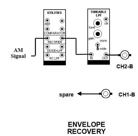
Procedure for Amplitude Demodulation

Connect AM output signal to an ideal envelope detector, modelled as per Figure above. For the low pass filter use the TUNEABLE LPF module. Your whole system might look like that shown modelled in Figure above.