Amplitude Modulation (AM) and Demodulation

Theory :

Amplitude modulation (AM) is the process in which the amplitude of a carrier wave, denoted as \( c(t) = \cos(2\pi f_c t) \), is varied in proportion to the message signal \( m(t) \). Mathematically, this is expressed as:

\( s(t) = A_c \left[ 1 + K_a m(t) \right] \cos(2\pi f_c t) \)

or equivalently:

\( s(t) = A_c \cos(2\pi f_c t) + A_c K_a m(t) \cos(2\pi f_c t) \)

where:

• \( A_c \) = carrier amplitude
• \( f_c \) = carrier frequency
• \( m(t) \) = message (modulating) signal
• \( K_a \) = amplitude sensitivity of the modulator
• \( s(t) \) = amplitude-modulated signal

Block Diagram for Amplitude Modulation

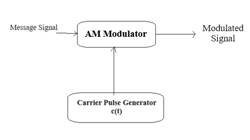
Fig 1: Amplitude Modulation

Modulation Index (\( \mu \))

The modulation index \( \mu \) quantifies how much the carrier amplitude varies in response to the message signal. It is defined as:

\( \mu = A_m / A_c \) or \( \mu = K_a A_m \), where:

• \( A_m \) = peak amplitude of the message signal \( m(t) \)
• \( A_c \) = carrier amplitude
• \( K_a \) = amplitude sensitivity

The modulation index determines modulation quality:

• \( \mu < 1 \): Under-modulation
• \( \mu = 1 \): 100% modulation (ideal)
• \( \mu > 1 \): Over-modulation (causes distortion)

Alternative definition: If \( K_a \) and \( A_m \) are unknown, \( \mu \) can be calculated from the modulated waveform:
\( \mu = \frac{A_{\text{max}} - A_{\text{min}}}{A_{\text{max}} + A_{\text{min}}} \)

• \( A_{\text{max}} \) = maximum amplitude of the modulated signal
• \( A_{\text{min}} \) = minimum amplitude of the modulated signal

Frequency Domain Description

The frequency-domain representation of an AM signal is obtained by applying the Fourier transform to \( s(t) \):

\( s(t) = A_c \left[ 1 + K_a m(t) \right] \cos(\omega_c t) \)

Applying Fourier transform and frequency-shifting properties:

\( S(j\omega) = \pi A_c [ \delta(\omega - \omega_c) + \delta(\omega + \omega_c) ] + \frac{1}{2} K_a A_c [ M(j(\omega - \omega_c)) + M(j(\omega + \omega_c)) ] \)

This spectrum consists of two impulses at ±\( \omega_c \) with amplitude \( \pi A_c \), plus two replicas of the message spectrum shifted to ±\( \omega_c \) and scaled by \( \frac{1}{2} K_a A_c \).

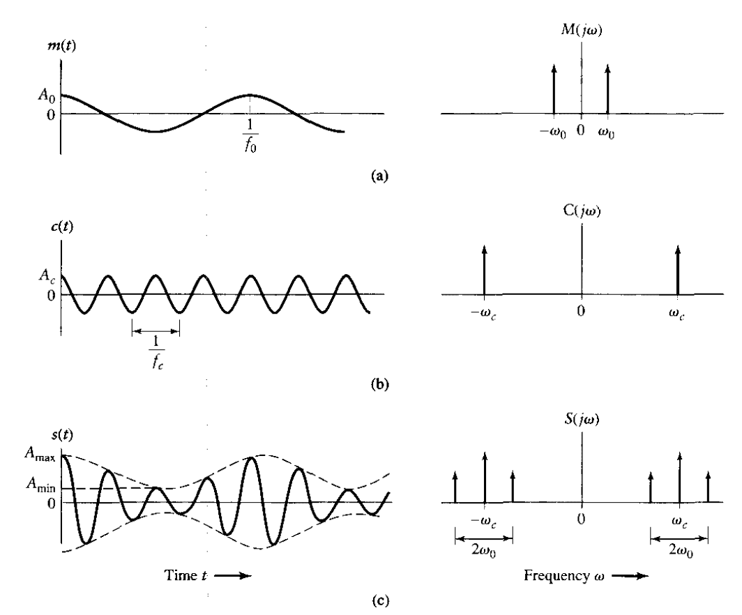
Fig 2: Time-domain (left) and frequency-domain (right) representation of AM with a sinusoidal message.

Bandwidth

The bandwidth of an AM signal is twice the highest frequency component of the message signal \( m(t) \):

BW = 2 * f_m

where \( f_m \) is the maximum frequency in the message signal.

Amplitude Demodulation

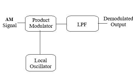
Fig 3: Amplitude Demodulation

Synchronous (coherent) demodulation recovers the original message signal. The AM input is:

\( s(t) = A_c \left[ 1 + K_a m(t) \right] \cos(2\pi f_c t) \)

• \( A_c \): carrier amplitude
• \( f_c \): carrier frequency
• \( m(t) \): message signal
• \( K_a \): amplitude sensitivity

Product Modulator (Multiplier)

Multiply \( s(t) \) with a locally generated carrier \( c(t) = \cos(2\pi f_c t) \):

\( v(t) = s(t) \cdot c(t) = A_c [1 + K_a m(t)] \cos^2(2\pi f_c t) \)

Using \( \cos^2\theta = \frac{1}{2}(1 + \cos2\theta) \):

\( v(t) = \frac{A_c}{2} [1 + K_a m(t)] + \frac{A_c}{2} [1 + K_a m(t)] \cos(4\pi f_c t) \)

The first term is the desired low-frequency component; the second term is a high-frequency component at \( 2f_c \).

Low-Pass Filter (LPF)

The LPF removes the high-frequency component while preserving the low-frequency message. The output is:

\( v_{LPF}(t) = \frac{A_c}{2} + \frac{A_c K_a}{2} m(t) \)

After DC removal and optional amplification, the original message signal \( m(t) \) is recovered.