Virtual Labs

SSB-SC Modulation

Theory

The SSB-SC modulated signal \( S(t) \) can be expressed as:

\( S(t) = \frac{A_c}{2} \left[ m(t) \cos(2\pi f_c t) \pm \hat{m}(t) \sin(2\pi f_c t) \right] \)

Where:

\( A_c \) is the amplitude of the carrier signal.
\( m(t) \) is the baseband (modulating) signal.
\( f_c \) is the frequency of the carrier signal.
\( \hat{m}(t) \) is the Hilbert transform of the modulating signal \( m(t) \).

In SSB-SC modulation, either the upper sideband (USB) or the lower sideband (LSB) is transmitted by choosing the corresponding sign (plus or minus) in the equation. The carrier \( A_c \cos(2\pi f_c t) \) is suppressed, and only one sideband is transmitted. This reduces the bandwidth required for transmission to half that of DSB-SC.

Block Diagram

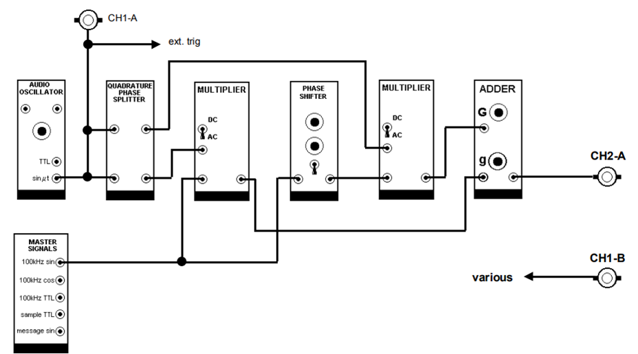
Figure 1

Procedures :

1. Before patching up an SSB phasing generator system, first examine the performance of the QUADRATURE PHASE SPLITTER module. With the oscilloscope adjusted to give equal gain in each channel it should show a circle. This will give a quick confirmation that there is a phase difference of approximately 90 degrees between the two output sine waves at the measurement frequency. Phase or amplitude errors should be too small for this to degenerate visibly into an ellipse. For the input signal source use an AUDIO OSCILLATOR module. For correct QPS operation the display should be an approximate circle. We will not attempt to measure phase error from this display
2. Vary the frequency of the AUDIO OSCILLATOR, and check that the approximate circle is maintained over at least the speech range of frequencies.
3. When satisfied that the QPS is operating satisfactorily, you are now ready to model the SSB generator. Patch up a model of the phasing SSB generator, following the arrangement illustrated in Figure above. Remember to set the on-board switch of the PHASE SHIFTER (perform 180 degree phase shift) to the ‘HI’ (indicates ‘high frequency range’) (100 kHz) range before plugging it in.
4. Set the AUDIO OSCILLATOR to about 1 kHz.
5. Switch the oscilloscope sweep to ‘auto’ mode, and connect the ‘ext trig’ to an output from the AUDIO OSCILLATOR. It is now synchronized to the message.
6. Display one or two periods of the message on the upper channel CH1-A of the oscilloscope for reference purposes. Note that this signal is used for external triggering of the oscilloscope. This will maintain a stationary envelope while balancing takes place. Make sure you appreciate the convenience of this mode of triggering. Separate DSBSC signals should already exist at the output of each MULTIPLIER. These need to be of equal amplitudes at the output of the ADDER. You will set this up, at first approximately and independently, then jointly and with precision, to achieve the required output result.
7. Check that out of each MULTIPLIER there is a DSBSC signal.
8. Turn the ADDER gain ‘G’ fully anti-clockwise. Adjust the magnitude of the other DSBSC, ‘g’, viewed at the ADDER output on CH2-A, to about 4 volts peak-to-peak. Line it up to be coincident with two convenient horizontal lines on the oscilloscope graticule (say 4 cm apart).
9. Remove the ‘g’ input patch cord from the ADDER. Adjust the ‘G’ input to give approximately 4 volts peak-to-peak at the ADDER output, using the same two graticule lines as for the previous adjustment
10. Replace the ‘g’ input patch cord to the ADDER. The two DSBSC are now appearing simultaneously at the ADDER output. Now use the same techniques as were used for balancing in the experiment entitled Modelling an equation in this Volume. Choose one of the ADDER gain controls (‘g’ or ‘G’) for the amplitude adjustment, and the PHASE SHIFTER for the carrier phase adjustment.
11. Balance the SSB generator so as to minimize the envelope amplitude. During the process it may be necessary to increase the oscilloscope sensitivity as appropriate, and to shift the display vertically so that the envelope remains on the screen.
12. When the best balance has been achieved, record results. Although you need the magnitudes P and Q, it is more accurate to measure (P and Q are Vmax and Vmin of the SSB-SC modulated signal)
a) 2P directly, which is the peak-to-peak of the SSB
b) Q indirectly, by measuring (P-Q), which is the peak-to-peak of the envelope.
13. As already stated, the TIMS QPS is not a precision device, and a sideband suppression of better than 26 dB is unlikely. You will not achieve a perfectly flat envelope. But its amplitude may be small or comparable with respect to the noise floor of the TIMS system. The presence of a residual envelope can be due to any one or more of:
• leakage of a component at carrier frequency (a fault of one or other MULTIPLIER )
• incomplete cancellation of the unwanted sideband due to imperfections of the QPS .
• Distortion components generated by the MULTIPLIER modules.
Any of the above will give an envelope ripple period comparable with the period of the message, rather than that of the carrier. Do you agree with this statement? If the envelope shape is sinusoidal, and the frequency is:
• Twice that of the message, then the largest unwanted component is due to incomplete cancellation of the unwanted sideband.
• The same as the message, then the largest unwanted component is at carrier frequency (‘carrier leak’)

•If it is difficult to identify the shape of the envelope, then it is probably a combination of these two; or just the inevitable system noise. An engineering estimate must then be made of the wanted-to-unwanted power ratio (which could be a statement of the form ‘better than 45 dB’), and an attempt made to describe the nature of these residual signals

• If not already done so, use the FREQUENCY COUNTER to identify your sideband as either upper (USSB) or lower (LSSB). Record also the exact frequency of the message sine wave from the AUDIO OSCILLATOR. From a knowledge of carrier and message frequencies, confirm your sideband is on one or other of the expected frequencies. To enable the sideband identification to be confirmed analytically you will need to make a careful note of the model configuration, and in particular the sign and magnitude of the phase shift introduced by the PHASE SHIFTER, and the sign of the phase difference between the I and Q outputs of the QPS (Quadrature Phase Shifter). I and Q are output terminals of QPS and Phase difference between then are 90 degree). Without these you cannot check results against theory

SSB-SC Demodulation

Block Diagram

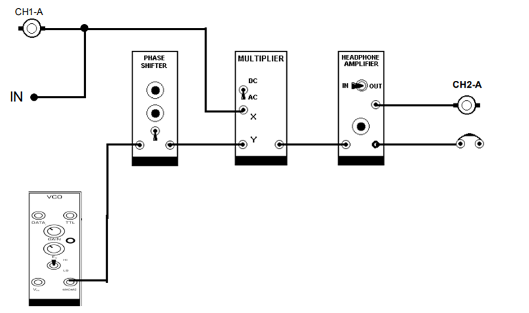
Figure 1

Procedures :

1. This is an asynchronous demodulation process. Here frequency of the VCO is adjusted with the frequency counter.
2. It is quite easy to make small frequency adjustments (fractions of a Hertz) by connecting a small negative DC voltage into the VCO Vin input, and tuning with the GAIN control.
3. Here, VCO facilitates fine tuning. Even if the frequency difference between the original carrier frequency (e.g., 100 KHz) and the frequency of the VCO differs by 10 Hz, then demodulated signal / speech will be quite intelligible
4. A recommended method of showing the small frequency difference between the VCO and the 100 kHz reference is to display each on separate oscilloscope traces - the speed of drift between the two gives an immediate and easily recognised indication of the frequency difference.
5. Connect an SSB signal, derived from speech, to the input ‘X’ of the multiplier as shown in the figure 1. Tune the VCO slowly around the 100 kHz region, and listen. Report results.