DSB-SC Modulation

Theory

Double Sideband Suppressed Carrier (DSB-SC) modulation is a type of amplitude modulation where only the sidebands are transmitted, and the carrier signal is suppressed. This method is more power-efficient compared to standard amplitude modulation (AM), as it eliminates the carrier, which does not carry useful information.

Mathematical Representation

The DSB-SC modulated signal \( S(t) \) can be expressed as:

\( S(t) = A_c m(t) \cos(2\pi f_c t) \)

Where:

• \( A_c \) is the amplitude of the carrier signal.
• \( m(t) \) is the baseband (modulating) signal.
• \( f_c \) is the frequency of the carrier signal.

In DSB-SC modulation, the carrier signal \( \cos(2\pi f_c t) \) is multiplied by the modulating signal \( m(t) \), resulting in the modulated signal \( S(t) \). The key characteristic of DSB-SC is that the carrier \( A_c \cos(2\pi f_c t) \) is not transmitted. Instead, only the sidebands generated by the multiplication of \( m(t) \) and \( \cos(2\pi f_c t) \) are transmitted.

Block Diagram

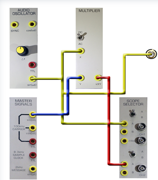
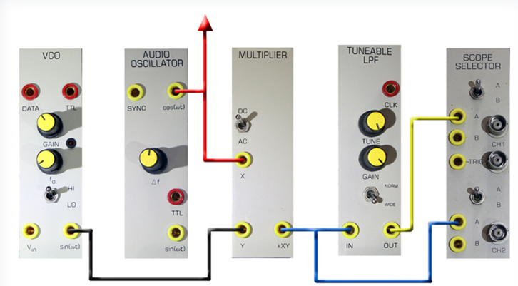
Figure 1

Procedures :

1. Patch up the arrangement of Figure 3.
2. Use the FREQUENCY COUNTER to set the AUDIO OSCILLATOR to about 1 kHz.
3. Measure and record the amplitudes A and B of the message and carrier signals at the inputs to the MULTIPLIER.
4. DSBSC = k A.cosμt B.cosωt .
5. Now peak to peak amplitude of the DSBSC signal will be 2*K.A.B volts.
6. Here 'k' is a scaling factor, a property of the MULTIPLIER. One of the purposes of this experiment is to determine the magnitude of this parameter.
7. Measure the peak-to-peak amplitude of the DSBSC. Since you have measured both A and B already, you have now obtained the magnitude of the MULTIPLIER scale factor 'k'; thus:
k = (dsbsc peak-to-peak) / (2 A B); Note that 'k' is not a dimensionless quantity
8. For showing the fine detail inside the DSBSC by Oscilloscope it is necessary that ‘µ’ be a sub-multiple of ‘ω’
9. Insert a BUFFER AMPLIFIER in one or other of the paths to the MULTIPLIER, and increase the input amplitude of this signal until overload occurs.
10. Now if you pass the DSB-SC signal thru the 60 KHz ‘LOWPASS LPF’ module then it result in no output as message frequency itself is 1 KHz. So, upper and lower side bands are 99 KHz and 101 KHz respectively
11. Now we’ll use VCO to generate carrier signal at our convenience.
12. Adjust the VCO frequency to about 10 kHz .
13. Set the AUDIO OSCILLATOR to about 1 kHz.
14. Set the front panel GAIN control of the TUNEABLE LPF so that the gain through the filter is unity.
15. Analysis predicts that the DSBSC is centred on 10 kHz, with lower and upper side frequencies at 9.0 kHz and 11.0 kHz respectively. Both side frequencies should fit well within the pass-band of the TUNEABLE LPF, when it is tuned to its widest pass-band, and so the shape of the DSBSC should not be altered.
16. Set the front panel toggle switch on the TUNEABLE LPF to WIDE, and the front panel TUNE knob fully clockwise. This should put the pass-band edge above 10 kHz. The pass-band edge (sometimes called the ‘corner frequency’) of the filter can be determined by connecting the output from the TTL CLK socket to the FREQUENCY COUNTER. It is given by dividing the counter readout by 360 (in the ‘NORMAL’ mode the dividing factor is 880).
17. Note that the pass-band GAIN of the TUNEABLE LPF is adjustable from the front panel. Adjust it until the output has a similar amplitude to the DSBSC from the MULTIPLIER (it will have the same shape). Record the width of the pass-band of the TUNEABLE LPF under these conditions.
18. Assuming the last Task was performed successfully this confirms that the DSBSC lies below the pass-band edge of the TUNEABLE LPF at its widest. You will now use the TUNEABLE LPF to determine the sideband locations.
19. The cut-off frequency of this LOWPASS FILTER can be varied using the TUNE control. Two frequency ranges, WIDE and NORMAL, can be selected by a front panel switch. The GAIN control allows signal amplitudes to be varied if required.
20. NORMAL range provides more precise control over the lower audio band, used for telecommunications message channels. The WIDE range expands the filter’s range to above 10 kHz.
21. Lower the filter pass band edge until there is a just-noticeable change to the DSBSC output. Record the filter pass band edge as fA. You have located the upper edge of the DSBSC at (w + μ) rad/s.
22. Lower the filter pass-band edge further until there is only a sine wave output. You have isolated the component on (ω - μ) rad/s. Lower the filter pass band edge still further until the amplitude of this sine wave just starts to reduce. Record the filter pass band edge as fB.

---

DSB-SC Demodulation

DSBSC Demodulation :

Recovering the message signal from the demodulated signal is performed coherently. That is, the demodulated signal is multiplied by a high-frequency sinusoid in perfect synchronization (in phase and frequency) with the incoming carrier.

This requirement poses a challenge on the design of the demodulator circuit, as it would then require a part for carrier-recovery. Failing to accomplish perfect synchronization will result in phase mismatch or frequency mismatch, leading to some form of distortion in the recovered signal.

Multiplying the modulated signal with a local carrier will produce a baseband signal as well as a signal modulated at double the carrier frequency. Therefore, a LPF is needed at the far end of the demodulator to recover the baseband signal .

DSBSC Demodulation Block Diagram

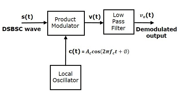
Fig. DSB-SC Demodulation Block Diagram

Procedures :

1. Use the same carrier signal used in DSBSC modulation, multiplier and a Tunable LPF to demodulate the DSBSC generated during DSBSC modulation.

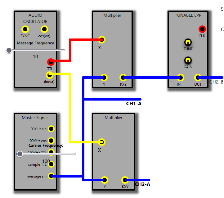
Fig. The TIMS Model of The Block Diagram of DSB-SC Demodulation

2. Switch the Scope Selector to CH1-A and CH2-B.
3. Observe the signal in time and frequency domains before and after the LPF simultaneously.
4. Vary the cutoff frequency of the LPF, and find the range of acceptable values for best recovery of the message.
5. Plot, in time, the best recovered signal you can obtain in your lab sheets.
6. Increase the cutoff frequency of the LPF beyond the range of good recovery.