SSB-SC Modulation

Theory

The SSB-SC modulated signal \( S(t) \) can be expressed as:

\( S(t) = \frac{A_c}{2} \left[ m(t) \cos(2\pi f_c t) \pm \hat{m}(t) \sin(2\pi f_c t) \right] \)

Where:

• \( A_c \) is the amplitude of the carrier signal.
• \( m(t) \) is the baseband (modulating) signal.
• \( f_c \) is the frequency of the carrier signal.
• \( \hat{m}(t) \) is the Hilbert transform of the modulating signal \( m(t) \).

In SSB-SC modulation, either the upper sideband (USB) or the lower sideband (LSB) is transmitted by choosing the corresponding sign (plus or minus) in the equation. The carrier \( A_c \cos(2\pi f_c t) \) is suppressed, and only one sideband is transmitted. This reduces the bandwidth required for transmission to half that of DSB-SC.

Block Diagram

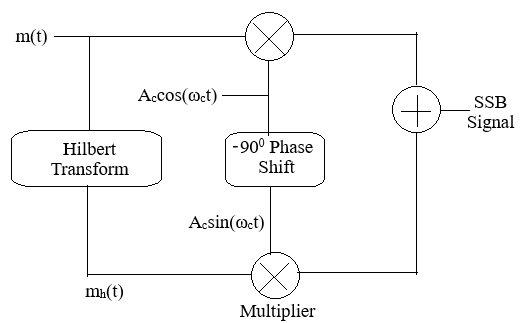
Fig: SSB-SC Modulation

Frequency Domain Description

The precise frequency-domain description of an SSB modulated wave depends on which sideband is transmitted. To investigate this issue, consider a message signal m(t) with a spectrum M(jω) limited to the band ω_a ≤ |ω| ≤ ω_m, as in the figure below.

The spectrum of the DSB-SC modulated wave, obtained by multiplying m(t) by the carrier wave A_c cos(ω_ct), is shown in the figure below. The upper sideband is represented in duplicate by the frequencies above ω_c and those below –ω_c; and when only the upper sideband is transmitted, the resulting SSB modulated wave has the spectrum shown in the figure below.

Likewise, the lower sideband is represented in duplicate by the frequencies below ω_c (for positive frequencies) and those above –ω_c (for negative frequencies); and when only the lower sideband is transmitted, the spectrum of the corresponding SSB modulated wave is as shown in the figure below.

Thus the essential function of SSB modulation is to translate the spectrum of the modulating wave, either with or without inversion, to a new location in the frequency domain. Moreover, the transmission bandwidth requirement of an SSB modulation...

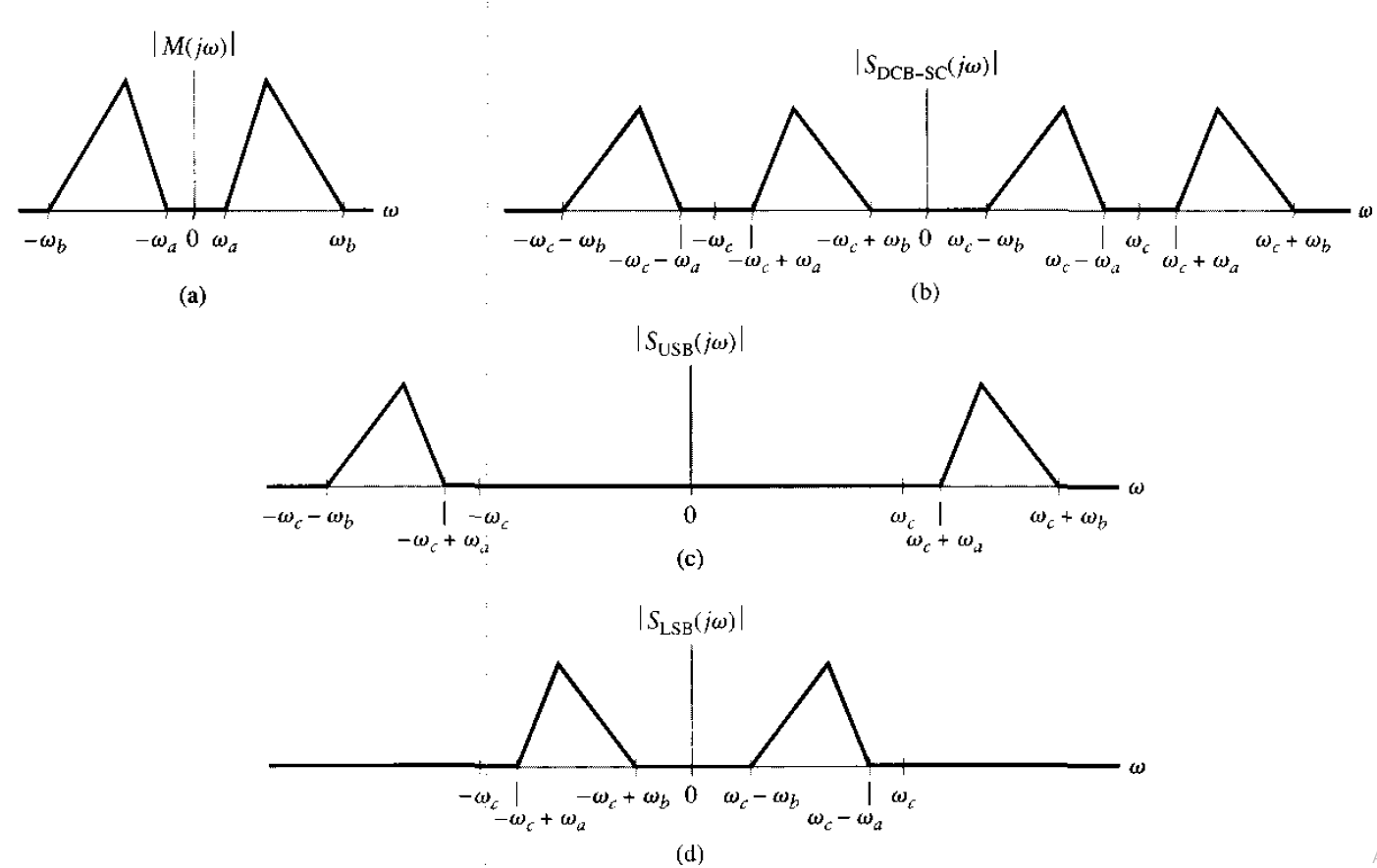
Fig: Frequency-domain characteristics of SSB modulation. (a) Magnitude spectrum of message signal, with energy gap from −ωₐ to ωₐ. (b) Magnitude spectrum of DSB-SC signal. (c) Magnitude spectrum of SSB modulated wave, containing upper sideband only. (d) Magnitude spectrum of SSB modulated wave, containing lower sideband only.

SSB-SC Demodulation

Block Diagram

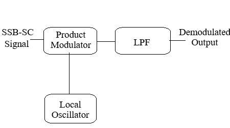
Fig: SSB-SC Demodulation

Demodulation using Coherent Detection

To retrieve \( m(t) \), the SSB-SC signal is multiplied with a coherent carrier:

\( S(t) \cdot 2 \cos(2\pi f_c t) \)

Substituting for \( S(t) \):

\( 2 S(t) \cos(2\pi f_c t) = A_c m(t) \cos^2(2\pi f_c t) \pm A_c \hat{m}(t) \sin(2\pi f_c t) \cos(2\pi f_c t) \)

Using trigonometric identities:

• \( \cos^2(2\pi f_c t) = \frac{1 + \cos(4\pi f_c t)}{2} \)
• \( \sin(2\pi f_c t) \cos(2\pi f_c t) = \frac{1}{2} \sin(4\pi f_c t) \)

This simplifies the expression to:

\( S(t) \cdot 2\cos(2\pi f_c t) = \frac{A_c}{2} m(t) + \frac{A_c}{2} m(t) \cos(4\pi f_c t) \pm \frac{A_c}{2} \hat{m}(t) \sin(4\pi f_c t) \)

Low-Pass Filtering

The components \( \cos(4\pi f_c t) \) and \( \sin(4\pi f_c t) \) lie in the high-frequency range. A low-pass filter removes these, leaving only:

\( \frac{A_c}{2} m(t) \)

Finally, scaling by \( \frac{2}{A_c} \) gives the original message signal \( m(t) \).