DSB-SC Modulation

Theory

Double Sideband Suppressed Carrier (DSB-SC) modulation is a type of amplitude modulation in which only the sidebands are transmitted while the carrier is suppressed. Let the message signal \( m(t) \) be band-limited to a bandwidth \( B \). This method is more power-efficient than conventional amplitude modulation (AM), since the carrier does not convey useful information. The total transmission bandwidth required for DSB-SC modulation is \( 2B \).

Mathematical Representation

The DSB-SC modulated signal \( s(t) \) can be expressed as:

\( s(t) = A_c m(t) \cos(2\pi f_c t) \)

Where:

• \( A_c \) is the amplitude of the carrier signal.
• \( m(t) \) is the baseband (modulating) signal.
• \( f_c \) is the frequency of the carrier signal.

In DSB-SC modulation, the carrier signal \( \cos(2\pi f_c t) \) is multiplied by the modulating signal \( m(t) \), resulting in the modulated signal \( s(t) \). The carrier component \( A_c \cos(2\pi f_c t) \) is not transmitted. Instead, only the sidebands generated by this multiplication are transmitted.

Block Diagram

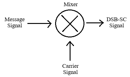
Fig 1: DSB-SC Modulation

Frequency Domain Description

Here, \( \omega_c = 2 \pi f_c \) is the carrier's angular frequency in radians per second. Using \( \omega \) in the frequency-domain representation simplifies mathematical expressions, especially for Fourier transforms, derivatives, and integrals. The relationship between angular frequency \( \omega \) and linear frequency \( f \) is \( \omega = 2\pi f \).

The frequency-domain representation of the DSB-SC signal is:

\( S(j\omega) = \frac{A_c}{2} \left[ M(j(\omega - \omega_c)) + M(j(\omega + \omega_c)) \right] \)

• \( S(j\omega) \) is the Fourier transform of the modulated signal \( s(t) \).
• \( M(j\omega) \) is the Fourier transform of the message signal \( m(t) \).
• The message spectrum is shifted to \( \pm \omega_c \).
• Both upper sideband (USB) and lower sideband (LSB) are present.
• The carrier component is suppressed.

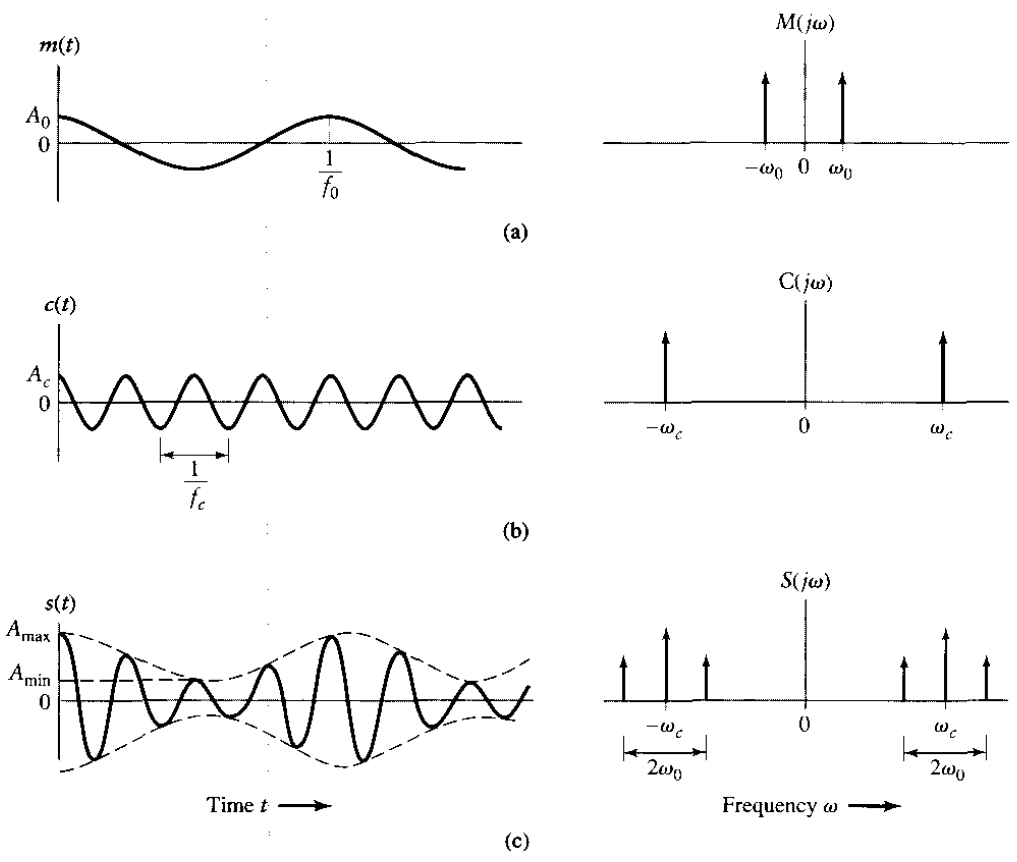
Fig 2: Time-domain (on the left) and frequency-domain (on the right) characteristics of DSB-SC modulation produced by a sinusoidal modulating wave. (a) Modulating wave. (b) Carrier wave. (c) DSB-SC modulated wave.

---

DSB-SC Demodulation

Block Diagram

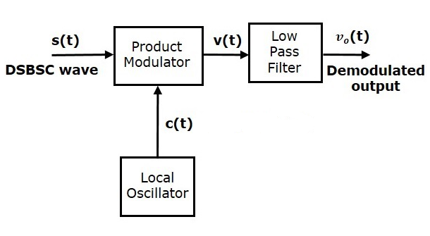
Fig 3: DSB-SC Demodulation

DSB-SC Demodulation

Recovery of the message signal is performed using coherent detection. The received signal is multiplied by a locally generated carrier that is perfectly synchronized in both phase and frequency with the incoming carrier.

The received signal is multiplied by a coherent carrier:

\( s(t)\cos(2\pi f_c t) = A_c m(t)\cos^2(2\pi f_c t) \)

Using the trigonometric identity:

\( \cos^2(\theta) = \frac{1}{2}(1 + \cos(2\theta)) \)

This simplifies to:

\( = \frac{A_c}{2} m(t) + \frac{A_c}{2} m(t)\cos(4\pi f_c t) \)

The second term represents a high-frequency component centered at \( 2f_c \), which is removed using a low-pass filter (LPF). The output of the filter is:

\( \hat{m}(t) = \frac{A_c}{2} m(t) \)

After appropriate scaling, the original message signal \( m(t) \) is recovered. Any mismatch in phase or frequency between the local oscillator and the carrier results in distortion in the recovered signal.