
Virtual Labs
IIT Kharagpur

Simulation
Virtual Labs
IIT Kharagpur
Simulation
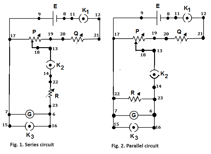
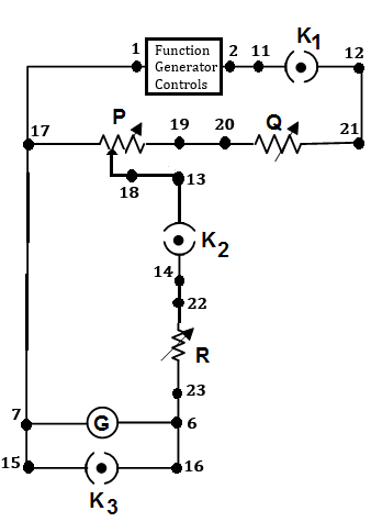


 17
18
19
17
18
19
 20
21
20
21
 22
23
22
23
| Sl No. | No. of oscillations | Time (sec) | Time period |
|---|---|---|---|
| Average Time period (T) = | |||
| Sl No. | P (ohm) | d (cm) | Deflection (θ) (rad) | Ig (A) |
|---|
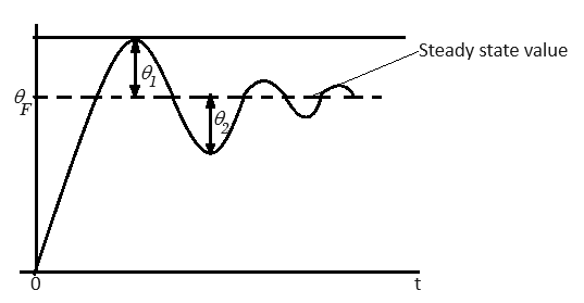
| Sl No. | R (ohm) | $$\delta = \delta_0 + \frac{G^2}{R \ 2\sqrt{JK}}$$ | θpeak (rad) | θsteady-state (rad) | $$\% \ Maximum \ overshoot = \frac{\theta_{peak} - \theta_{steady-state}}{\theta_{steady-state}} \times 100$$ |
|---|
| Sl No. | Frequency (Hz) | ω (rad/s) | δ | Amplitude (cm) |
|---|